Food system challenges in rural forested communities

There is increasing awareness of food access and availability challenges in so-called food deserts (too little available food) or food swamps (too much low-quality food). One helpful geographical insight from prior research is that as cities expand into surrounding countryside, new retail developments follow, and big grocery stores are often to be found in the suburbs or beyond the city limits, while inner city grocery stores close as wealth and population density decline (Hamidi 2020).

My team has been looking at the complexities of food accessibility at the urban-rural interface, particularly in rural regions with substantial forest cover. While cities have sprawled into surrounding countryside, formerly remote rural areas have been pulled into new relationships with cities, in the form of commuting (Olson and Munroe 2012), or as new “bedroom” communities for city dwellers who want a more rural lifestyle, or as a weekend “getaway” to recreate in nearby forests (Munroe et al. 2017, van Berkel 2014).

Figure 1: Main thoroughfare in Shawnee, Perry County Ohio. Population 319 in 2019. Photo Credit Darla Munroe

In 2017-2018, I interviewed a variety of community key informants in an Appalachian Ohio study area[1], comprising of small towns in Athens, Hocking and Perry counties. Though my central focus was on small town resilience to big employment shocks (Morzillo et al. 2015), the complexities of food in this region were a common theme among respondents. These towns have often surprising mixtures of high poverty, significant forest tourism, and small group business initiatives. Specifically, Athens County, Ohio, is trying to capitalize on new biking trails where weekend cyclists from all over the state come to ride hard and then drink craft beer. Schools are promoting entrepreneurship, encouraging students to create sustainable livelihood strategies for themselves via food trucks, farm-to-table programs or other such small-scale ventures.

At the same time, grocery options in small towns can be limited. Many communities do not have a dedicated grocery store, and they must rely on what’s obtainable at the convenience store if driving to the Kroger in the next town over is not an option. Public transportation is particularly limited in Appalachian Ohio; the rural poor often locate in places where walking to a post office to collect benefits is possible, and thus are limited to whatever food options might be available in these village centers. Within the state or even larger region, if you are laid off from your job, you might move to a town where you have a family connection, however distant. These areas offer a rural quality of life, and a low cost of living, which appeals to rich and poor alike.

Figure 2: Downtown Glouster in Athens County Ohio. Population 1896 in 2019. Photo Credit Darla Munroe

As a geographer, it is hard to see small towns reorienting their economic development strategies to cater to (relatively) wealthy tourists while locals are dependent on whatever the local dollar store might carry. At the same time, I marvel in the complexity of these urban-rural spaces (Irwin et al 2009) that defy easy categorization and rather call for much deeper collaboration and engagement. For those students in the 6th grade onward who are being taught that their economic futures are, at least in part, in their own hands and subject to their own imaginations, I can’t wait to see what this landscape might yield in decades to come.

Darla Munroe

Professor and Chair

Department of Geography, The Ohio State University


References

Hamidi, S. (2020). Urban sprawl and the emergence of food deserts in the USA. Urban Studies57(8), 1660-1675.

Irwin, E. G., Bell, K. P., Bockstael, N. E., Newburn, D. A., Partridge, M. D., & Wu, J. (2009). The economics of urban-rural space. Annu. Rev. Resour. Econ.1(1), 435-459.

Morzillo, A. T., Colocousis, C. R., Munroe, D. K., Bell, K. P., Martinuzzi, S., Van Berkel, D. B., … & McGill, B. (2015). “Communities in the middle”: Interactions between drivers of change and place-based characteristics in rural forest-based communities. Journal of Rural Studies42, 79-90.

Munroe, D., Gallemore, C. & Van Berkel, D. (2017). Hot Tub Cabin Rentals and Forest Tourism in Hocking County, Ohio. Revue économique, 3(3), 491-510. https://doi.org/10.3917/reco.683.0491

Olson, J. L., & Munroe, D. K. (2012). Natural amenities and rural development in new urban‐rural spaces. Regional Science Policy & Practice4(4), 355-371.

Van Berkel, D. B., Munroe, D. K., & Gallemore, C. (2014). Spatial analysis of land suitability, hot-tub cabins and forest tourism in Appalachian Ohio. Applied Geography54, 139-148.


[1] This research was funded by USDA NIFA Award #2016-6701925177, Biodiversity, ecosystem services, and the socioeconomic sustainability of rural forest-based communities, 2016-2021


The Food Environment Doesn’t Impact Your Health…Unless You Use It

A lot of public attention has focused on so-called “food deserts.” These are food environments that lack low-priced healthy food options, and are often identified as areas that lack a full-service supermarket. (See Figure 1 for a map of Ohio.)

I have argued elsewhere that I prefer not to use the popularized terms of “food deserts” or “food swamps.” Food deserts suggest a lack of food, when these locations, particularly urban locations, often have a plethora of unhealthy food. Further, the terms “desert” and “swamps” are not asset-based approaches to characterizing community members’ residential locations.

Poor food environments are disproportionately found in poor urban and rural communities and communities of color. These communities are also associated with relatively higher levels of poor mental and physical health outcomes, such as greater levels of stress, diet-related disease, and insecurity [1-4].

Figure 1. USDA’s Low income, Low Access Census Tracts (previously termed “food deserts”) [7]

While an increasing amount of public funds at the federal, state and local level aim to improve food environments with the hopes of improving diet, many researchers have dismissed any significant relationship between the food environments and diet. There are two reasons for the lack of consistent and significant findings: (1) the way people go about measuring the food environment, and (2) people do leave poor food environments for better ones, particularly if they have a car, enough time and money, and feel safe (e.g., not going to face personal racism)[5].

A recent study lead by my advisee and PhD candidate, Alannah Glickman, and co-authored by myself and Darcy Freedman, addressed these issues by studying how people use their immediate food environment, rather than assuming everyone uses the space in the same way [5].  This gets to a fundamental way in which to conceptualize space [6]: as absolute – envision two convenience stores and one grocery store in a neighborhood; as relative – think about the position of the household relative to stores and the distance households travel; and as relational – how do households use the stores in their neighborhood. Nearly all research focuses on the second approach; we focus on the third.

Using a novel approach applied to two Ohio neighborhoods (Figure 2), we found that there is a significant relationship between the food environment and diet if people shop in their immediate, poor food environments. For people who do more than 50% of their shopping within their poor food environments, we found, all else equal, an eight point decrease in their healthy eating index (which is measured on a 100-pt. scale; the average American’s score is 58.7).

Figure 2. These are two images of the food environment taken in our study areas – Columbus, Ohio (left) and Cleveland, Ohio (right) [Google maps]

In my position now as an associate professor in the John Glenn College of Public Affairs, I ask questions, such as: is there a public purpose to intervene in the food environment? However, to understand the complexities of the food environment, I returned to my training in geography!


Jill Clark, Associate Professor

John Glenn College of Public Affairs


References Cited

  1. Walker, R.E., C.R. Keane, and J.G. Burke, Disparities and access to healthy food in the United States: A review of food deserts literature. Health & Place, 2010. 16(5): p. 876-884.
  2. Caspi, C.E., et al., The local food environment and diet: a systematic review. Health & place, 2012. 18(5): p. 1172-1187.
  3. Clifton, K.J., Mobility Strategies and Food Shopping for Low-Income Families A Case Study. Journal of Planning Education and Research, 2004. 23(4): p. 402-413.
  4. Ver Ploeg, M., Access to affordable and nutritious food: updated estimates of distance to supermarkets using 2010 data. 2012: United States Department of Agriculture, Economic Research Service.
  5. Glickman, A., J.K. Clark, and D. Freedman, Residential Proximity to Low-Quality Food Retailers and Diet Behavior: Exploring the Micro Food Environment within Low-Income Neighborhoods, in Association of Public Policy Analysis and Management. 2020: Virtual.
  6. Harvey, D., Social Justice and the City 1973, London: Edward Arnold
  7. USDA. Food Access Research Atlas. 2020 [cited 2021 February 22]; Available from: https://www.ers.usda.gov/data-products/food-access-research-atlas/go-to-the-atlas/.


Food Access: A Time Issue

In the US, the rising obesity rate and obesity-related comorbidities, such as cardiovascular diseases and Type-II diabetes, have drawn health geographers’ attention. It is generally understood that the lack of access to healthy food provisioning, such as grocery stores selling fresh fruits and vegetables, is driving this obesity crisis. Under this context, the US Department of Agriculture (USDA) Economic Research Service (ERS) develops an inquiry tool, the Food Access Research Atlas (1), generally known as the “food desert locator,” to highlight areas with both low-income and limited access to grocery stores. The tool also incorporates other variables, such as car-ownership, to identify communities at risk of food insecurity.

“Food deserts” identified by the USDA Food Access Research Atlas (1)


This spatial approach, however, has raised questions about the etiology of obesity. It has been found that the correlation between healthy food access and healthy diets is not statistically consistent and is somewhat insignificant (2). In order to articulate the health effects of the community food environment, health geographers argue that other non-spatial variables need to be considered. One such variable is time.

Time shapes food access in two dimensions. On the one hand, the time component, or “temporality,” manifests in the urban food system (3) — grocery stores have different opening hours, farmers’ markets operate in different seasons. For example, it is found that grocery stores in downtown Columbus, Ohio, although there are many of them, close relatively early than stores located in the suburb. This disparity in space-time access to food is visualized by a 3D Geographical Information System (GIS) (4). The plentiful spatial access but limited temporal access could be explained by the store type (e.g., mostly privately owned) and the relatively high crime rate in the downtown neighborhood. Since downtown stores have limited operating hours, local residents may restrict their food choices and could be subject to diet-related health consequences. On the other hand, time shapes individuals’ mobility to procure food. People burdened with multiple social roles, such as childcare while raising an income, may find themselves less available to procure healthy food (5). A study using a travel diary survey identifies that the difference in time use exists between genders and among different races. Full-time employed women and African Americans are at the disadvantage of having less discretionary time (6). The lack of time may victimize these vulnerable social groups and expose them to food insecurity.

A 3D visualization of space-time food access in Columbus (4)


Thus, food access is not only a spatial issue but also a temporal issue. Employing a spatial approach alone to evaluate food access is insufficient. Other tiers of non-spatial variables, such as time, should be factored in to produce knowledge about food access equity and justify the health effects of community food environments.

Xiang Chen

Department of Geography

University of Connecticut

Xiang Chen is an Assistant Professor in the Department of Geography, University of Connecticut, USA. He received a Ph.D. in Geography at The Ohio State University (2014). His research is focused on GIScience, community health, and food accessibility.


  1. https://www.ers.usda.gov/data-products/food-access-research-atlas/go-to-the-atlas.aspx
  2. Caspi, C. E., Sorensen, G., Subramanian, S. V., & Kawachi, I. (2012). The local food environment and diet: A systematic review. Health & Place, 18(5), 1172-1187.
  3. Widener, M. J., & Shannon, J. (2014). When are food deserts? Integrating time into research on food accessibility. Health & Place, 30, 1-3.
  4. Chen, X., & Clark, J. (2016). Measuring space-time access to food retailers: a case of temporal access disparity in Franklin County, Ohio. The Professional Geographer, 68(2), 175-188.
  5. Rose, D., & Richards, R. (2004). Food store access and household fruit and vegetable use among participants in the US Food Stamp Program. Public Health Nutrition, 7(8), 1081-1088.
  6. Kwan, M. P. (2002). Feminist visualization: Re-envisioning GIS as a method in feminist geographic research. Annals of the Association of American Geographers, 92(4), 645-661.


Would global trade contribute to food security without overwhelming our planet?

Global trade supplies food to countries in conditions of food scarcity by redistributing food commodities among the different regions of the world; at this time, roughly one-fourth of the food supply globally is provided through international trade (D’Odorico et al., 2014). If more productive regions (producing more output per unit input of land) export their produce to countries with lower productivity, we could feed more people than we could when the food supply is only domestically generated. As shown in Figure 1, for example, cereal demand in Africa and East Asia can hardly be met without global trade. The global food trade is also a more efficient way of using natural resources world-wide. 588m3 of water is needed to produce 1 ton of wheat in France, whereas 18,698m3 of water is required for producing the same amount of wheat in Somalia (Mekonnen & Hoekstra, 2011). By importing agricultural commodities, countries with low agricultural productivity and scarce natural resources like Somalia can optimize resource use (i.e., water or land) at both the national and global level. Thus, the global food trade not only plays an important role in global food security, but has also become a crucial part of allocating limited global resources.

Figure 1. Global Cereal Trade in 2017. The colors of the regions represent the net import of cereal products (import-export). Reds are net importers and blues are net exporters. The top 10 flows in terms of the volume traded are shown. The flows shown account for 16.3% of the total cereal products related to global trade. Cereals include wheat, rice, maize, barley, millet, oat, rye, and sorghum. Trade data were taken from the FAOSTAT database.


However, global trade is not always conducive to global food security and resource conservation.

First, decreased food prices due to trade can boost consumption in the importing countries, thus in turn causing overproduction in the exporting countries (Kastner et al., 2014). The so-called rebound effect highlights a possibility that increased production efficiencies through trade may increase overall demand, so that resource use can instead be expanded. For example, deforestation in the Brazilian Amazon has been driven by the increase in soybean production for livestock feed in developing countries, with a rebound of soybean prices in global markets (Morton et al., 2006).

Second, trade dependency can make importing countries vulnerable to external shocks, as these countries increasingly rely on resources that they do not directly control (D’Odorico et al., 2014). It is widely known that droughts in production regions, as well as banned grain exports, triggered the Arab Spring in 2011[i]. An unexpected crisis like the pandemic last year (and continuing into this year) poses greater challenges to import-dependent countries as well[ii]. Furthermore, an influx of cheap subsidized commodities from exporting countries can threaten both the domestic market and local biodiversity, as well as undermine rural livelihoods, which in turn strengthens the trade dependency (Carr et al., 2016). For instance, exports of maize from the U.S. to Mexico under NAFTA are reported to be as detrimental to Mexico’s smallholder farmers and domestic biodiversity of maize varieties (Martinez-Alier, 1993).

Third, the increasing export of value-added crops (i.e., coffee, cocoa, or tropical fruits) from lower-income countries may influence food security at the local level. The increasing rate of traded volume from 1987 to 2017 is higher in stimulants (244%) and fruits (217%) than in cereals (153%), which has been largely driven by developing countries. While some argue that cultivating such crops is beneficial to food security because of increase in rural income (Kuma et al., 2016), others find negative relationships between household food security and value-added crop production (Anderman et al., 2014). For example, the expansion of banana plantations in Northern Laos for Chinese customers raises concerns about food security due to the conversion of paddy rice fields to the plantation and rising rice prices (Friis & Nielsen, 2016).

The three points listed above imply that “a multifaceted and linked global strategy” (Godfray et al., 2010) should complement international food trade in order to feed growing populations without overwhelming our planet. Measures to shift dietary preferences toward less consumption of meat products can be helpful for mitigating the rebound effect. Continuous efforts to increase domestic productivity and to diversify suppliers will buffer external supply shocks in import-dependent countries. Strategies to ensure the food security of cash crop farmers in developing countries are required, and environmental regulations for sustainable resource use need to be implemented as well.

Sohyun Park

PhD Candidate in Department of Geography

The Ohio State University


  • Anderman, T. L., Remans, R., Wood, S. A., DeRosa, K., & DeFries, R. S. (2014). Synergies and tradeoffs between cash crop production and food security: A case study in rural Ghana. Food Security, 6(4), 541–554.
  • Carr, J. A., D’Odorico, P., Suweis, S., & Seekell, D. A. (2016). What commodities and countries impact inequality in the global food system? Environmental Research Letters, 11(9), 095013.
  • D’Odorico, P., Carr, J. A., Laio, F., Ridolfi, L., & Vandoni, S. (2014). Feeding humanity through global food trade. Earth’s Future, 2(9), 458–469.
  • Friis, C., & Nielsen, J. Ø. (2016). Small-scale land acquisitions, large-scale implications: Exploring the case of Chinese banana investments in Northern Laos. Land Use Policy, 57, 117–129.
  • Godfray, H. C. J., Beddington, J. R., Crute, I. R., Haddad, L., Lawrence, D., Muir, J. F., Pretty, J., Robinson, S., Thomas, S. M., & Toulmin, C. (2010). Food security: The challenge of Feeding 9 Billion People. Science, 327.
  • Kastner, T., Erb, K.-H., & Haberl, H. (2014). Rapid growth in agricultural trade: effects on global area efficiency and the role of management. Environmental Research Letters, 9(3), 034015.
  • Kuma, T., Dereje, M., Hirvonen, K., & Minten, B. (2016). Cash crops and food security: Evidence from Ethiopian smallholder coffee producers. The Journal of Development Studies, 55(6), 1267-1284.
  • Martinez-Alier, J. (1993). Distributional Obstacles to International Environmental Policy: The Failures at Rio and Prospects after Rio. Environmental Values, 2(2), 97–124.
  • Mekonnen, M. M., & Hoekstra, A. Y. (2011). The green, blue and grey water footprint of crops and derived crop products. Hydrology and Earth System Sciences, 15(5), 1577–1600.
  • Morton, D. C., DeFries, R. S., Shimabukuro, Y. E., Anderson, L. O., Arai, E., Del Bon Espirito-Santo, F., Freitas, R., & Morisette, J. (2006). Cropland expansion changes deforestation dynamics in the southern Brazilian Amazon. Proceedings of the National Academy of Sciences of the United States of America, 103(39), 14637–14641.


[i] https://www.pbs.org/newshour/world/world-july-dec11-food_09-07

[ii] https://www.brookings.edu/blog/future-development/2020/07/14/middle-east-food-security-amid-the-covid-19-pandemic/

Agricultural Risks to Changing Snowmelt

Snowpacks store cold water in winter, which is later melted in warmer spring months to produce streamflow. Historically, irrigated agriculture has relied on snowmelt runoff as an important seasonal water supply in many regions across the world, such as the western United States.

However, Climate change has already begun to change the spatial and temporal patterns of snowmelt runoff — causing a decreasing magnitude of snowfall and earlier melting of snowpacks. Consequently, irrigated agriculture, which has been depending on snowmelt runoff happening with a certain magnitude, at a specific time, and in a given location, are exposed to potentially important risks under a warming climate.

Although such changes in snowmelt-derived water resources are often cited as a key threat to irrigated agriculture and global food security, previous studies have focused on annual changes in runoff, without resolving the sub-annual changes in water supply and crop-specific water demand.

To characterize such risks, we differentiate surface water supply from three sources: snowmelt runoff, rainfall runoff, and alternative water supply such as inter-basin water transfer. Comparing monthly surface water supply with surface water demand under both the historical climate (1985-2015) and predicted warming scenarios (2°C and 4°C above pre-industrial conditions), we identify where irrigated agriculture has been mostly depending on snowmelt runoff in the past 30 years. Also, we find basins in high-mountain Asia (the Tibetan Plateau), central Asia, central Russia, the western U.S., and the southern Andes are particularly vulnerable to decreasing snowmelt availability in crops’ growing seasons due to a future warming climate.

Therefore, these most risky basins will require increasing additional water supplies by increasing inter-basin transfer, pumping additional groundwater, or consuming water required for other uses. Notably, providing those additional water supplies may sometimes cause additional environmental and social problems, thus improved irrigation practices or crop switching may be needed to ensure food security under changing snowmelt.

Yue Qin

Assistant Professor, Department of Geography

The Ohio State University

Uncertainty Problems and Census Data: The 2020 Census & Exurbanization Example

Last year, I had opportunities to learn about the 2020 Census from a research seminar and a professional meeting to promote Complete Count of the 2020 Census. As you may have heard already, there are some new characteristics in the 2020 Census as below (U.S. Census Bureau, n.d.-a, n.d.-c, n.d.-b):

  • The 2020 Census will be the first to offer options for internet and phone responses.
  • There will be a greater reliance on technology to prepare for and execute the count.
  • The 2020 Census will update its Master Address File (MAF) and ensure that every living quarter in the U.S. is included in the census universe by collaborating with state and local governments and using aerial imaging software.
  • For enhanced enumeration, Census takers will be equipped with smart devices, and data will be collected digitally in real-time.
  • There are no questions about citizenship on the 2020 Census.
  • Responses for the Census will never be shared with agencies of immigration or law enforcement.
  • The country is experiencing a period of heightened fear and deliberate misinformation.

Potential Uncertainty in the 2020 Census

Most of the characteristics above seem to be helpful to produce more accurate Census data. On the other hand, there might be some potential uncertainty in the 2020 Census data. First, there are some challenges to being counted on the Census data, including language barriers, mistrust in government, privacy/cybersecurity concerns, physical barriers such as inaccessible multifamily units, untraditional living arrangements, and lack of reliable broadband or internet access. Second, there may exist hard-to-count (HTC) groups for the Census, including children under five years old, racial and ethnic minorities, limited English proficiency households, immigrants, renters and residents who often move, alternative or overcrowded housing units, gated communities and publicly inaccessible multifamily units, persons displaced by natural disasters, persons experiencing homelessness, young mobile adults, and single-parent headed households (The City of Stillwater, Payne County, OK, n.d.). Thus, the 2020 Census may provide enhanced accuracy of the data and also uncertain data for some criteria of the Census.

Example of Uncertainty in Visualizing Exurbanization

Due to the potential uncertainty in the Census data, some geographic inquiries that utilize the Census data may reveal the uncertainty problems, such as visualizing the location of exurban areas. Simply speaking, the exurban areas have characteristics between urban and suburban areas. There are multiple different definitions of exurbanization in literature, and the location of certain exurban areas on maps may vary depending on the definition (Ban & Ahlqvist, 2009). In specific, you can visualize the exurbanization of certain areas by using the Census data, geospatial data, and fuzzy-set approach (Ban & Ahlqvist, 2009; Fisher, 2000; Wechsler et al., 2019; Zadeh, 1965), and could create a map that represents different degrees of exurbanization (Figure 1). In Figure 1, the degree of exurbanization of Los Angeles County, CA is visualized based on the definition of exurbanization in (Daniels, 1999). According to Daniels (1999), the exurban areas are defined using value ranges of some attributes, including population, distance from a major urban center, commuting distance, and population density. The definitions of Daniels (1999) themselves include semantic uncertainty due to the vagueness and the ambiguity (see Ban & Ahlqvist (2009) for details). However, in this blog, we will focus on the population attribute of the exurbanization definition. As mentioned above, the potential uncertainty in 2020 Census data may introduce another type of uncertainty, the error (Fisher, 2000). Most of the definitions of exurbanization use the population attribute (Berube et al., 2006). It is likely that the results of the visualization of exurbanization may present uncertainty in the locations of exurban areas.

Figure 1. Visualization of the degree of exurbanization of Los Angeles County, CA based on the exurban definition from Daniels (1999). (A) shows boundaries of exurban areas in crisp, non-fuzzy membership and (b) in the fuzzy-set membership (reproduced from Figure 16.5 of Wechsler et al. (2019)).

There would exist other geographical inquiries that might introduce uncertainty when dealt with the 2020 Census data. What would be the examples? Then how could the uncertainty problems be resolved? Things to ponder remains, and indeed, the initial process of thinking could be definitely uncertain.


References

  1. Ban, H., & Ahlqvist, O. (2009). Representing and negotiating uncertain geospatial concepts – Where are the exurban areas? Computers, Environment and Urban Systems, 33(4), 233–246. https://doi.org/10.1016/j.compenvurbsys.2008.10.001
  2. Berube, A., Singer, A., Wilson, J. H., & Frey, W. H. (2006). Finding Exurbia: America’s Fast-Growing Communities at the Metropolitan Fringe. 48.
  3. Daniels, T. (1999). When City and Country Collide: Managing Growth In The Metropolitan Fringe. Island Press.
  4. Fisher, P. (2000). Sorites paradox and vague geographies. Fuzzy Sets and Systems, 113(1), 7–18. https://doi.org/10.1016/S0165-0114(99)00009-3
  5. The City of Stillwater, Payne County, OK. (n.d.). Historically Hard to Count Populations. Retrieved November 30, 2020, from http://www.paynecountycensus.org/page/home/your-community-s-info/historically-hard-to-count-populations
  6. US Census Bureau. (n.d.-a). About the 2020 Census. The United States Census Bureau. Retrieved November 30, 2020, from https://www.census.gov/programs-surveys/decennial-census/2020-census/about.html
  7. US Census Bureau. (n.d.-b). Census.gov. Census.Gov. Retrieved November 30, 2020, from https://www.census.gov/en.html
  8. US Census Bureau. (n.d.-c). What Is the 2020 Census? 2020Census.Gov. Retrieved November 30, 2020, from https://2020census.gov/en/what-is-2020-census.html
  9. Wechsler, S., Ban, H., & Li, L. (2019). The Pervasive Challenge of Error and Uncertainty in Geospatial Data: Volume Eight (pp. 315–332). https://doi.org/10.1007/978-3-030-04750-4_16
  10. Zadeh, L. A. (1965). Information and control. 8(3), 338–353.

Hyowon Ban

Class of 2009, Associate Professor

Department of Geography

California State University, Long Beach


Subsidizing Luxury: Neoliberalism, Urban Redevelopment and the Geography of Educational Inequity

In recent decades, city governments have looked to neoliberal redevelopment policies to stimulate urban redevelopment and growth. Public private partnerships, tax increment financing zones and tax abatements are regular policy tools implemented to spur redevelopment in areas that have experienced substantial disinvestment. Redevelopment policies are critical in efforts to spur investment and population growth in neighborhoods that have lost population. But, little consensus exists to determine when is the appropriate time to end these incentive programs in neighborhoods. Should these tools still be used in areas where housing markets have rebounded and where signs of gentrification are evident?  While these tools are widely used and very popular among policymakers, a substantial body of research has found these neoliberal development strategies to reallocate public resources to the affluent while undermining traditional public institutions, such as schools, who rely heavily on property taxes for their financial needs.

Given that these redevelopment policies are most often targeted to urban neighborhoods that are served by schools with older infrastructure and greater student needs, neoliberal redevelopment policies can exacerbate the geography of educational inequity in metropolitan areas. Analysis by Good Jobs First has found that even accounting for poor data tracking, at least $1.8 billion in revenues were lost to public schools as a result of this policy in 2018 alone. The revenue lost could have funded an additional 27,000 teachers in these school systems. The influence of tax incentives on urban education in particular has spurred the topic of redevelopment policy to emerge within teacher union contract negotiations. Our recent research project sought to better understand the influence of residential tax incentives on the public education system in Columbus.

We focused our analysis on the city’s residential tax abatement program. While larger corporate tax abatements are often discussed in the media, very little attention is paid to residential tax abatements. The residential tax abatements provide 100% tax abatements for up to 15 years on residential properties built or substantially rehabbed in core urban neighborhoods. These incentives can be very important in fostering redevelopment for neighborhoods who are experiencing challenging market conditions. But some critics have questioned why abatements are still in place in neighborhoods that have experienced substantial redevelopment?

Our analysis sought to understand the characteristics of residential properties that were listed for sale or had been sold with a tax abatement in the prior 3 years. We researched MLS listings for the past three years building a database of residential properties sold or currently listed for sale with a residential tax abatement in the zip codes targeted for tax abatements.

Area map of study area and zip codes used for analysis

Our preliminary findings suggest that a very large proportion of the residential tax base is lost to through the abatement program. Properties with residential tax abatements are selling at costs much higher than nearby real estate values and are primarily only affordable to high wealth households. In short, the abatement program is subsidizing luxury housing at the expense of resources for public education in the city.

We identified 365 residential units with a tax abatement sold in the past three years (or currently listed for sale). These 365 residential units represented more than $132 million in taxable value, given the current structure of the residential tax abatement program, these properties would account for a loss of more than $130 million in tax base each year for the next 15 years. Hypothetically, even if property values did not increase, the cumulative cost of these 365 tax abated units over the course of 15 years would represent nearly $2 billion in property values that would go untaxed.

Tax abated properties are selling for much higher sales prices than local real estate values and are most likely only affordable to high wealth households. The average sales price for a 2-bedroom residential unit with a tax abatement was $434,000. A household would need at least $130,000 in annual income to afford the average tax abated 2-bedroom unit in the core of the city.

description of impacts of residential tax abatements

Figure 2: Summary of residential tax abated properties identified in our database of abated residential sales and listings.

In contrast, the median annual household income for families with children in these abatement areas is approximately $29,000. Residential abatements provide substantial cost savings to buyers and conversely loss of tax base for the school district. The highest price tax abated property was a 2-bedroom luxury condominium in the arena district which sold for $1.6 million.

Listing description and taxes paid for the most expensive residential tax abated property in our database (a 2-bedroom luxury condominium).

Figure 3: Listing description and taxes paid for the most expensive residential tax abated property in our database (a 2-bedroom luxury condominium).

The real estate taxes paid for this property was $3,100 in 2019, without the abatement the real estate taxes paid should have been more than $33,000. Thus, to subsidize this luxury condominium, the public tax base is denied more than $30,000 in taxes annually, for up to 15 years.

While it is still challenging to fully understand the effects of residential abatements on the fiscal health of the Columbus City Schools, early analysis finds some alarming trends in the long-term sustainability of the district’s tax base.

Columbus City Schools district taxable value per pupil (and state ranking) 1989 to 2019.

Figure 4: Columbus City Schools district taxable value per pupil (and state ranking) 1989 to 2019.

Data from the Ohio Department of Taxation indicates that Columbus City schools tax base is declining in contrast to other districts in the State of Ohio. When ranked against districts across the state based on the taxable value of property per pupil, Columbus City Schools was ranked 107th (out of 610 districts) in 1989 and in 2019 has fallen to ranking 423rd.

More importantly, these policies also represent an alarming disconnect between urban redevelopment policy and the sustainability of the Columbus City School district. While the abatement programs have helped spur an influx of high wealth households into abatement areas, they degrade the public resources available to the nearly 30,000 children (of which more than half live in households with income under the poverty line) in abatement areas. A diminished tax base means fewer resources to upgrade older school buildings, support the needs of students who need special services and programming within schools and impacts the district’s resilience in responding to the increased needs produced by the COVID-19 pandemic.

Our preliminary results suggest that these neoliberal development tools bolster the real estate market but at the expense of resources for children in these neighborhoods. While real estate sales have soared in these redeveloping areas, students in Columbus City schools contend with an under resourced school district. We call for a reforming urban redevelopment policies to be less focused on recruiting high wealth households and re-centered on meeting the needs of children within these core urban neighborhoods.


Jason Reece, Assistant Professor,

City & Regional Planning, Knowlton School


Victoria Abou-Ghalioum, Graduate Fellow,

School of Environment and Natural Resources

Administrative Data: Impacts on Decennial Census and Research

The Demographic Research area of the Center for Economic Studies (CES) within the U.S. Census Bureau is responsible for researching and developing innovative ways to use administrative records in decennial census and survey operations. Our team of demographers, economists, geographers, and sociologists evaluate a wide array of administrative data from other federal agencies, state governments, and third party organizations. We assess the quality and coverage of these datasets and investigate how they may be useful for the Census Bureau’s data collection and processing efforts.  In addition, we use linked census, survey, and administrative records data to conduct scholarly research and to create estimates that could not be created without linked data to better inform the American Public.

Much of the work we do hinges on the ability to link records for people across different data sources. We are able to do this because another area at the Census Bureau first uses personally identifiable information (PII), such as name, date of birth, etc., to assign anonymous unique identifiers to individuals in our census, survey, and administrative data sets. They then strip off all PII and provide an anonymized file that includes these unique identifiers to researchers like myself to investigate important research questions.

One type of analysis we often perform involves linking survey data to administrative records to see if responses to survey questions match what we find in administrative records for people found in both data sources. For example, my colleagues and I linked responses from the Current Population Survey (CPS) on Medicare coverage to Medicare enrollment data and measured the extent of survey misreporting of Medicare coverage.  In this study, we found that survey responses were mostly consistent with enrollment data but we did note a small undercount of Medicare coverage in the CPS. In another case, we linked responses by American Indians and Alaska Natives regarding Indian Health Service (IHS) coverage in the American Community Survey (ACS) to IHS Patient Registration data. With this study, we found much higher levels of discordance between survey responses and administrative records. While some of the differences we found were likely due in part to definitional differences between the data sources, our analysis also suggested true inconsistencies in reporting of Indian Health Service coverage.

We also use linked data to understand how people’s responses to decennial census and survey questions change over time. For example, we have examined responses to census and survey questions on race and Hispanic origin. In one study on American Indians and Alaska Natives, we found considerable changes in racial responses between the 2000 and 2010 censuses, and by linking individuals to their responses in ACS data we were able to evaluate the characteristics of those who changed their race and those who did not.  In another project we evaluated how people reported their Hispanic origin in the 2000 and 2010 censuses and the ACS and examined the characteristics associated with a change in response, including the impact of changes in question wording and other data collection aspects.

My current work uses linked survey and administrative records data to increase our understanding of participation in social safety net programs.  This work is part of a joint project between the Census Bureau and the U.S. Department of Agriculture’s Economic Research Service and Food and Nutrition Service, as well as multiple state partners.  States that participate in the project send us data on people that receive Supplemental Nutrition Assistance Program (SNAP), Women, Infants, and Children (WIC), as well as data on Temporary Assistance for Needy Families (TANF) benefits. We link these records to ACS data to estimate eligibility and participation in each of these programs by various demographic, socioeconomic, and household characteristics.  We send our estimates of eligibility and participation back to the states with the aim of providing data that can inform program administration. For example, if we find that a particular characteristic or geographic area is associated with high rates of eligibility for a particular program but low rates of participation, it may indicate the need for further outreach.

The team I work with recently developed a visualization displaying these estimates for a few states. The visualization allows users to examine WIC eligibility and participation rates among infants and children at the county level by various characteristics. We are currently developing a similar visualization for SNAP recipients, which will include both children and adults. This is an example of the estimates we can produce with blended data that provide the public with additional information.

Renuka Bhaskar is an OSU alumna and a senior researcher in the Center for Economic Studies at the U.S. Census Bureau. Any opinions and conclusions expressed herein are those of the author and do not represent the views of the U.S. Census Bureau.

Making Sense of Census Data Resources

In my role as Ohio State’s Geospatial Information Librarian, a lot of the work that I do is related to helping researchers – at all levels and across a wide variety of disciplines – think through how they can locate, analyze, and visualize geographic data. And a lot of the time, data products provided by the U.S. Census Bureau will be relevant for addressing the research questions that they are asking.

When we hear the word “census” in 2020, our thoughts likely turn to the decennial census, and for good reason. It is hard to overstate the importance of the 2020 Census in terms of political representation and federal funding allocation, and the ways these will impact our communities over the next decade.

But it’s also important to note that census data products cover a lot more than the decennial census. In fact, the U.S. Census Bureau conducts more than 130 different surveys and programs, including the American Community Survey (ACS), Current Population Survey (CPS), Economic Census, and Longitudinal Employer-Household Dynamics (LEHD) program, to name a few.

More recently, the U.S. Census Bureau has also been releasing a variety of interesting experimental data products, which are described as “innovative statistical products created using new data sources or methodologies that benefit users in the absence of other relevant products.” Two that garnered some attention earlier this year and that have recently gone through a second phase are the Household Pulse Survey and Small Business Pulse Survey, which provide data about the social and economic effects of the COVID-19 pandemic on American households and businesses, respectively.

As mentioned in an earlier post, data products from the U.S. Census Bureau are free and publicly available. Here are a few different ways you can access these data for research, teaching, or class assignments:

U.S. Census Bureau

A lot of census data products are directly accessible in data.census.gov, a new platform that replaced American FactFinder in early 2020. The platform features a new search interface aimed at making it easier for users to locate the data they need, with more datasets planned to be added over time. It’s also possible to browse and download data tables for various programs by topic and year. If you are unable to find the data you are looking for through either of those options, you can always go directly to the website for the specific program you are interested in to see what data access options are available (and see here for the list of all surveys and programs). TIGER data products are also publicly available for working with census data in a GIS.

data.census.gov is the U.S. Census Bureau’s new platform for facilitating data access

IPUMS

IPUMS is a great resource for accessing a number of historical and contemporary census data products not readily available elsewhere. For example, NHGIS – the National Historical Geographic Information System – provides access to summary data tables and GIS-compatible boundary files from 1790 to the present and for all levels of U.S. census geography. For those working internationally, IPUMS also recently announced the launch of IHGIS – the International Historical Geographic Information System – with data tables and GIS-compatible boundary files from population, housing, and agricultural censuses from a number of countries, with more to be added over time.

Up to this point, all of the data resources I’ve been discussing have been more focused on providing summary data, presented in aggregate at different levels of U.S. census geography. But various IPUMS products also provide access to historical and contemporary census microdata, that is, individual records containing information collected about persons or households. IPUMS USA, for example, provides access to harmonized microdata from decennial censuses from 1850 to 2010 and American Community Surveys from 2000 to the present, though geographic information for these records is limited compared to summary data. IPUMS also recently announced the release of the Multigenerational Longitudinal Panel (MLP), which links individuals’ records between censuses spanning 1900-1940, with plans to extend back to 1850 in the future.

All IPUMS data products are free and publicly available, though there is a registration process required before gaining access to these data.

IPUMS provides access to various unique historical and contemporary census data products

Licensed Resources

In addition to the public data resources described above, the University Libraries licenses several resources that provide access to census data products in a fairly user-friendly way, especially for beginners. PolicyMap and Social Explorer are two examples, both of which include interactive map viewers that facilitate some geographic exploration of the data without the need to download and import data into a GIS every time. I have worked with instructors in various departments who have incorporated one of these databases into an assignment or recommended them as data sources for student projects. One other important note about Social Explorer is that it includes data tables for the 1970, 1980, 1990, and 2000 decennial censuses normalized to the 2010 census geographies to facilitate longitudinal comparisons, with data available down to the tract level.

Social Explorer has a number of interactive map viewers for exploring census data variables

This list of census data resources is by no means exhaustive, but I hope it will be a good starting point for those looking to use census data products for research, teaching, or class assignments. Have fun exploring these resources, especially if you are new to census data or less familiar with some of the other surveys and programs conducted by the U.S. Census Bureau. And if you are having trouble finding the data you need or have other questions, you can always contact a librarian.

Joshua Sadvari

Assistant Professor, Geospatial Information Librarian

University Libraries

The Ohio State University

Map Production to Support 2020 Census Programs and Operations

Maps have always played a significant role in conducting a census. This post discusses map production within the Geography Division of the U.S. Census Bureau to support the 2020 Census.

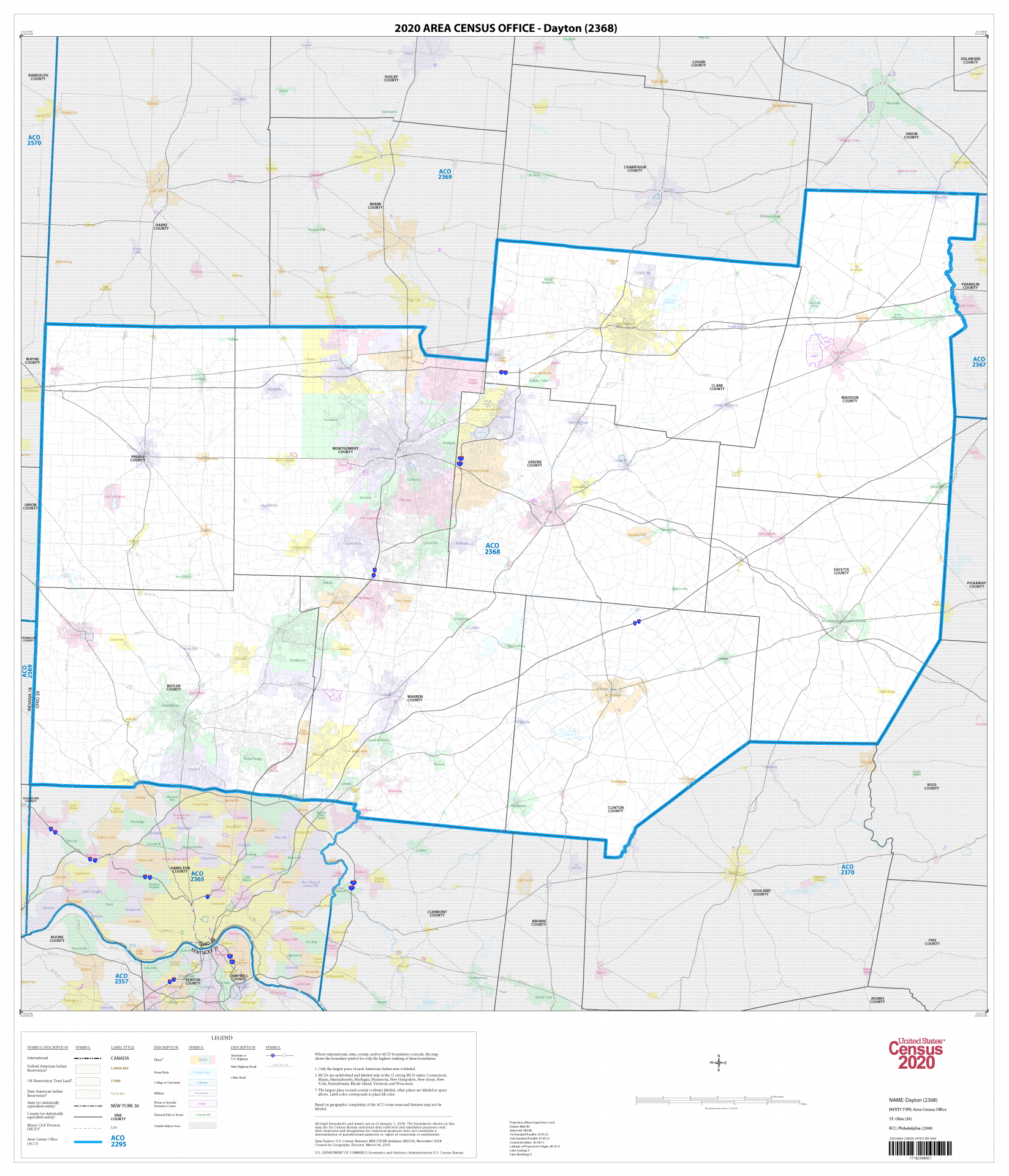
Although most of the field operations for the 2020 Census were conducted on digital instruments rather than paper, there is still a need for paper maps to support many operations. For instance, staff in the area census offices (ACOs) use large-format paper maps to help understand and visualize the boundaries of the collection geographic areas within their ACO or to visualize the workload for a particular operation. Other operations, such as Remote Alaska, Update Enumerate, and the Island Areas Census, are conducted entirely on paper. In these cases, staff use small-format maps to locate their workloads and annotate updates in the field.

In order to provide the number of maps required for geographic programs and field operations under strict production timelines, the Census Bureau utilizes the Census Automated Map Production System (CAMPS). CAMPS is automated mapping software that runs in a batch environment. CAMPS was developed in the lead up to the 2010 Census and continues to be a major part of production mapping. Cartographers design maps by setting up project parameter tables that describe everything from the title that will appear on a map to the appearance of labels and features for each feature class that will appear on a map. During peak operations, CAMPS creates thousands of map sheets per hour. For example, for the Local Update of Census Addresses Operation (LUCA), CAMPS created more than 800,000 unique map sheets over an 11 day period!

Largely due to the digital nature of many 2020 Census operations, most operations requested that we create large-format maps on as few sheets as possible, preferably a single sheet for each mapping entity. This presented some design challenges as CAMPS traditionally scales maps to as many sheets as needed based on the density of a particular geographic type within the subject area. Due to the large variety of the sizes of the subject areas for some map types, we designed multiple scale-dependent parameter configurations for each map type. Figure 1 shows a map of the Dayton ACO. This map was created in CAMPS and identifies the boundaries of the ACO. This map type included maps with scales as small as 1:1,000,000 and as large as 1:11,000 for the ACOs in the contiguous U.S.

Although we created the vast majority of our 2020 Census field maps in CAMPS, we also used commercial mapping software to produce maps, using manual interactive design and scripting. We designed map document templates in the commercial mapping software and developed scripts to automate the creation of the maps. For the Island Areas Census, we created approximately 5,600 basic collection unit (BCU)-based maps with imagery. Figure 2 shows an example of one of these maps in Guam, which was used in the field along with additional small-format maps to conduct the Island Areas Census.

Web maps and web map applications have also become a large part of our work for the 2020 Census. Web maps are particularly valuable for the communication of 2020 Census concepts to the general public and our partners. We developed web map applications to aid in outreach efforts in hard-to-count communities with the Response Outreach Area Mapper and to indicate how the Census Bureau planned to conduct the census with the Type of Enumeration Area Viewer, the In-Field Address Canvassing Viewer, and the Mail Contact Strategies Viewer. We were able to communicate with the public about the participation of local partners in programs such as LUCA, the Participant Statistical Areas Program, and the New Construction Program. In addition, we found the web map applications to be useful for the internal tracking of the status and progress of programs.

We are currently planning and developing maps and cartographic products for the next phase of the 2020 Census: data dissemination.

Kevin Hawley is an OSU alumnus and chief of the Cartographic Products and Services Branch in the Geography Branch at the U.S. Census Bureau. Any views expressed are those of author and not necessarily those of the U.S. Census Bureau.


You can see more of Kevin Hawley’s important work and its basis in Geography below.