For those interested, here is a link to a recent Resources For the Future podcast about our recent book “Reversing Deforestation: How Market Forces and Local Ownership are Saving Forests in Latin America.”
Click here.
For those interested, here is a link to a recent Resources For the Future podcast about our recent book “Reversing Deforestation: How Market Forces and Local Ownership are Saving Forests in Latin America.”
Click here.
My colleague Doug Southgate and I released our book titled Reversing Deforestation: How Market Forces and Local Ownership are Saving Forests in Latin America through Stanford University Press in late 2024. We of course invite all of you to have a look. It can be obtained through Stanford University Press, or Amazon. Additionally, Doug and I will be presenting a webinar on January 22, 2025.
We argue that forests in Latin America (and elsewhere) are at an inflection point because of trends in population, technology, and local ownership. All are bending in the right direction. For instance, growth in demand for food is slowing at the same time food production per hectare is hitting all-time highs. A key reason that food production has risen so much in Latin America is local ownership of farmland, which encourages investments in new technologies and higher yields. Local ownership – which includes individual ownership as well as community and Indigenous ownership – has also been expanding across the region’s forests, providing new opportunities for protection, planting, and natural regeneration.
In the book, we describe how we got to the point of converting 350 million treed hectares in Latin America (0.9 billion acres) to food production over the last 170 years. Population growth was the key driver. Human numbers increased from around 30 million in Latin America in 1850 to over 650 million today. Most of this increase happened because death rates fell as nutrition improved, medical advances occurred (including vaccines and antibiotics) and sanitation got better, among other things.
Today, population growth is slowing rapidly, not because calamity is upon us, as the authors of The Limits to Growth predicted in the early 1970s, but instead because people are controlling themselves. Just as birth rates fell years ago in Europe, North America, and other wealthy countries, they are now down across Latin America. As a result, the total fertility rate – the average number of children per woman – has fallen to 1.9, lower than the replacement rate. Population will continue to grow for a while in the region but is expected fall back nearly to today’s levels of 650 million by the end of the century.
Other factors contribute to deforestation, including government policies like open access, road building, and subsidies meant to expand agriculture and increase population in the hinterlands. Mining and logging play a role, but modestly in comparison.
As Nobel Prize winner Norman Borlaug showed us, adding land is not the only way to enhance food production. Increasing yields also works. Fittingly, the roots of the Green Revolution, which raised crop yields in developing countries last century, lie in Latin America.
Yes, nearly half of all tropical deforestation last century happened in Latin America, however, intensification reduced it. Since 1961, Brazil added 48 million hectares to corn and soybean production, an area bigger than the U.S. state of California. Yet if corn yields had not risen 268% and soybean yields 191%, Brazil would have needed 2.5 times that much land to produce the same quantity.
Because of intensification, real commodity prices for corn, soybeans, wheat, and rice have fallen since the 1960s. They are likely to fall further as slowing population growth meets new technology for food production.
As helpful as these trends are for slowing deforestation, they may not reverse it for the simple fact that government owns most of the forests in Latin America. In North America and Europe, governments do a great job of controlling access to public forests, although their management leaves substantial room for improvement. Through large swaths of government owned forests in Latin America, government agencies have trouble discouraging conversion to agriculture.
A well-recognized solution to de facto open access like this is ownership. Places like Chile and Costa Rica have developed land registries and encouraged individual land ownership, so deforestation has already reversed there. But thanks to Nobel Prize winner Elinor Ostrom, we have come to recognize that ownership can happen in lots of different ways, not just the fee simple ownership that many in North America and Europe are used to. When local ownership is considered broadly, it turns out that it is expanding across Latin America.
Early last century, land redistribution in Mexico created community forests called ejidos, which are well managed and resistant to deforestation. As a result, Mexico’s deforestation rate is low. Guatemala established several types of community forests in the Maya Biosphere Reserve in the late 1990s, which have become models for people all over the world. Deforestation rates within the community forests are slower than deforestation rates outside of them, and they are far slower than deforestation rates in some national parks in Guatemala. Brazil has been designating land in the Amazon for Indigenous communities as well, increasing local ownership and with it, opportunities for forest protection.
Ownership provides numerous benefits for forests. Although people do a better job maintaining forests when they have an ownership stake, carbon emissions and biodiversity losses are externalities, so even on locally owned land there will still be too much deforestation and too little afforestation. But private transactions – Payments for Environmental Services (PES) – can be deployed more effectively on private land. Nowadays, lots of companies are seeking opportunities to prevent forest loss or regenerate forests, and they prefer working with private owners than governments.
The evidence is pretty clear that forest planting is far more widespread on private land than public land. Natural regeneration is a perfectly valid way for forest renewal to proceed, but planting results in more stock more quickly. So from a carbon perspective, planting is beneficial.
When we look at the data and trends on people, technology, and ownership, Doug and I are incredibly optimistic about the future of forests in Latin America, and the entire world. Population and technology are heading in the right direction. In many places, the institutions of ownership are also heading in the right direction too, but now is a good time refocus our attention on local ownership, strengthening it where necessary.
Have a look at this piece published in The Conversation:
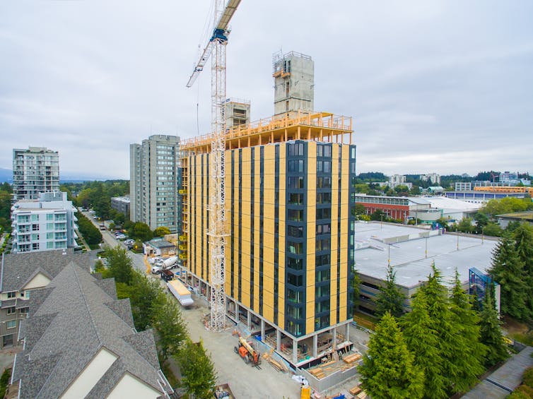
High rises made out of wood? What matters in whether ‘mass timber’ buildings are sustainable
by Brent Sohngen
A material that’s been around since people built shelters – wood – is increasingly being proposed for low- and mid-rise buildings.
Companies behind these “mass timber” projects say that wood is a lower-carbon alternative to steel or concrete and brings other benefits, such as faster construction time and lower cost than concrete and steel. Advocates say the wood materials, made of compressed layers of wood with glue, offer good fire safety as well.
As an economist who studies forestry and natural resources, I took an interest in this building trend when I heard that a local bar on campus was going to be replaced by a 13-story building made out of wood.
I see any increase in the use of wood in buildings as positive for reducing the substantial carbon footprint of buildings. But it is critical to consider where wood is sourced and whether forests are managed sustainably.
One way that researchers assess the environmental footprint of a product or service is called a life-cycle analysis, which calculates the cradle-to-grave impact.
One life-cycle analysis found that using mass timber in a 12-story building in Oregon had an 18% lower global warming impact compared with constructing the building with steel-reinforced concrete. The carbon emissions benefits are even greater when comparing timber with steel for low- and mid-rise buildings. In these studies, the global warming benefits mostly result from lower emissions in sourcing, transporting and manufacturing the material for these large wood buildings, compared with steel or concrete components, rather than efficiencies in heating or cooling or disposal of the materials at the end of the building’s lifespan.
On a global level, the raw material for mass timber – forests – absorb large amounts of carbon dioxide from the atmosphere, making them an important carbon “sink.”
Tree cutting is one of the most widespread disturbances in forests, yet, after accounting for all harvesting, fires, land use change and other disturbances, forests in the United States still remove a net 754 million tons of CO2 per year from the atmosphere, an amount equivalent to 13.5% of U.S. emissions. Globally, the picture is similar, with forest growth removing 2.6 billion tons of CO2 more from the atmosphere than the combined effect of all wood harvesting, deforestation, forest fires and other disturbances.
Although today forests are a net CO2 sink in the U.S. – taking in more carbon from the atmosphere than released through disturbance – before the middle of the last century, they were a big source of carbon emissions. Back then, farmers converted land to agriculture, foresters cut old-growth trees to produce lumber, and forest fires raged. Carbon losses in the U.S. were so large that land-based emissions around the turn of the 20th century were on par with emissions from deforestation in tropical regions today.
Over the past 100 years, the trend has reversed, as forests have removed far more CO2 from the atmosphere than they have released. One reason for this transition has been a sustained increase in crop yields, which has allowed for greater farm output on fewer acres. As a result, grain prices fell in real terms and farmers abandoned less productive lands, allowing forests to return. These regrowing forests, in turn, removed carbon from the atmosphere.
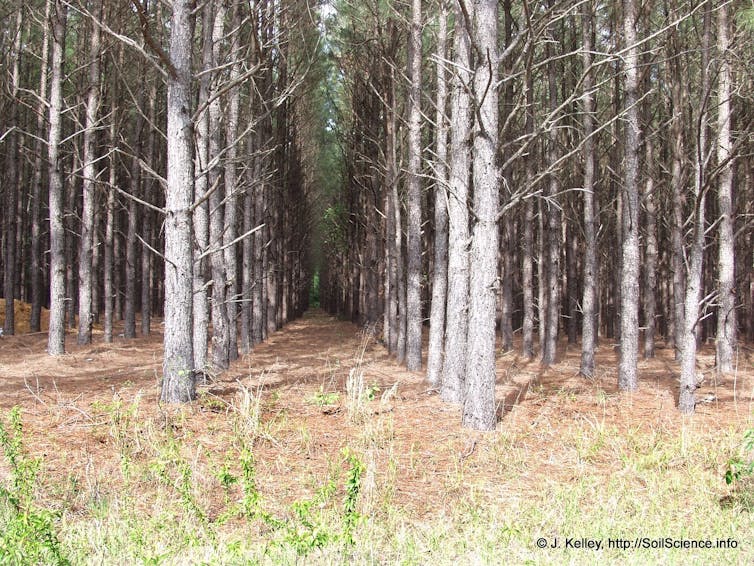
Abandonment was not the only reason trees regrew in the U.S. Even as foresters were still sawing their way through old-growth stocks in the first half of the 1900s, some foresighted forest landowners began planting trees because timber scarcity was growing, as evidenced by timber prices rising at 3% to 4% per year. By the 1950s and 1960s, over a million acres were being planted annually in the U.S., and today, the area planted is double that.
To examine whether wood is sustainably sourced, rather than contributing to higher carbon emissions, it is instructive to consider the economics of forest management.
A shift toward using wood rather than other materials in low- to mid-rise building designs will drive demand for wood products, resulting in both more harvesting and more planting. Any increase in harvesting carries risk, including an increase in carbon emissions, habitat loss, and other impacts. Perhaps the most evident effects happen when surging demand causes logging in sensitive ecosystems, critical habitats or old-growth forests. If lost, ecosystem services like biodiversity are often impossible to replace.
Carbon may be less of a worry because it can be returned to forests through regrowth. However, some critics maintain that harvests deposit CO2 in the atmosphere for the period between a timber harvest and forest regrowth, resulting in a massive CO2 emission.
There is considerable debate about this “excess” emissions hypothesis. Other research into the effects of increased wood demand illustrates that both harvesting and regeneration increase when demand rises. When timber investments are modeled alongside harvesting, carbon stocks in forested lands increase when wood demand ratchets up. This finding is not new. The example of the last century reveals that elevated timber demand and higher wood product prices strengthen incentives for landowners to intensively manage commercial forests – plant more acres, improve varieties, shift species mixes, fertilize, control drainage and manage competition.
The sustainability of mass timber will also be determined by which forests supply this new demand. It is unlikely that much of this new harvesting will happen on the 42% of U.S. forests owned by various units of government.. Many of these forests are either administratively protected – for example, as a wilderness area – or are remote and costly to access. Where cutting is allowed, logging is slowed by the considerable planning, impact assessment and public involvement required.
Even many private landowners have gotten into the habit of protecting for the purpose of environmental services. Today, over 37 million acres of private land in the U.S. are enrolled in conservation easements, which limit what current and future owners can do with their land. Not all of these protected lands are forests, but where they are, new demands for mass timber are unlikely to result in more harvesting.
Aside from these legally protected lands, forest protection happens in many private forests simply because many forest owners are inattentive or they have strong preferences for wildlife and benefits other than timber revenue. As a result, research has found that nonindustrial landowners as a whole are unlikely to expand cutting even if demand does grow substantively.
At the other end of the spectrum, industrial interests own just 20% of U.S. forests, but supply 46% of the nation’s timber. An overwhelming share of these forests are managed intensively with plantations. Tree planting is so prevalent that industrial owners account for 60% of private planted forests, defined as those that are artificially regenerated via planting or seeding.
Intensive management explains how so few industrial forests can support such expansive harvesting. If demand rises, these owners will have strong incentives to increase harvests. Yet because forests are a valued asset, they will also grow more and bigger trees with new plantings and intensified management.
One effect of climate change on forestry is that rising carbon dioxide levels have increased forest growth through higher rates of photosynthesis. A 2022 paper I co-authored found that elevated levels of CO2 had a particularly large effect on wood volume in younger, planted stands. Not only did forest plantations contain more wood volume at the same age than natural stands, but our study estimated that over the past 50 years, planted stands gained 62% more volume from this carbon “fertilization”. The number of trees per acre did not change substantively over this same time period, so most of this wood volume increase resulted in bigger trees.
Between 1997 and 2017, industrial owners accounted for eight out of every 10 new hectares of planted forests on private land as they doubled plantation area. No one will confuse these forests for old-growth forests, but from a commercial perspective, planted trees have become the lowest cost source of timber. They also relieve pressure on natural stands.
More critically for the atmosphere, expanding the area of young, fast-growing stands enhances the overall carbon sink of forests and brings an incentive to manage forests that serve the built environment.
I recently took my blog post “Why are Nature-Based Carbon Offset Prices So Low?” and used a new feature in Google’s NotebookLM to create an 8 minute podcast of the written post. The podcast is not all that bad actually, outside of mangling my name in a few places. In fact, the language model comes up with a few ways of discussing carbon offsets that make the points better than I did originally. Have a listen here.
Brent Sohngen (Ohio State University; sohngen.@osu.edu); Justin Baker (North Carolina State University); Adam Daigneault (University of Maine), and Alice Favero (RTI, International)
UPDATE (09/25/2024): We have published a paper on SSRN based on this blog posting, but the paper contains additional tests and analysis of GTM. That paper can be downloaded here.
Summary
Sections in this report
This turned out to be a longer response than we expected, so for easier reading, here are links to the sections in the report. These section headings should allow individuals who want to review our response to a specific issue raised by Searchinger and Berry without reading the entire document. Click here for a pdf of this document.
Approaches to Analyze the Carbon Implications of Wood Harvesting
No human activity counterfactual
Structural Bias Due to Parameter Extrapolation
Introduction
Recently, Tim Searchinger and Steven Berry have published a report through WRI making numerous claims about the carbon implications of wood harvesting. Their article is a response to our comment (available here) on the CHARM model, which we wrote and sent to Nature as a “Matters Arising” submission. That exchange is under review.
In their response to our criticisms of CHARM, Searchinger and Berry make several assertions and claims about the carbon implications of wood harvesting in general and the Global Timber Model (GTM) in particular. While our criticism of CHARM focuses on deficiencies in the approach taken by CHARM, Searchinger and Berry (the latter was not an author on the original CHARM paper, but apparently should have been?) take GTM to task. In this response to their response, we reiterate fundamental points about carbon accounting and forests, and we set the record straight on mistakes they have made in their interpretation of GTM and several of its parameters.
We start with the basic claim in Searchinger and Berry that the question of carbon neutrality in harvested wood products is a purely physical question – having nothing to do with economics. The carbon intensity of any product is a function of the inputs, management decisions, and technologies used to produce those products. The choice of technology, supplier, and other factors are all at their heart economic decisions. In forestry, the carbon intensity of wood is a function of its production process, including how a forest is managed. It just so happens that for forest products, a big chunk of the production process happens in nature and that part has an outsized influence on the carbon intensity of wood products.
We do not believe that there is any way to divorce the question of carbon neutrality in wood products from economics – especially natural resource economics. Models used to conduct the analysis or project future changes in forest sector carbon sinks and emissions sources must integrate natural processes (ecology, atmospheric exchange) with economic systems (markets and resource management dynamics). This brings us to the different world view of GTM (natural resource economics) and Searchinger and Berry’s CHARM model (purely physical). It turns out that this difference in world view has an outsized influence on the outcomes of the two approaches, so we start by describing this difference. We then tackle some of the claims Searchinger and Berry make about GTM.
World View
The easiest way to understand differences in how these two groups view wood consumption and forest management can be illustrated with a figure (figure 1), which displays key big picture differences in the Searchinger and Berry/CHARM world view (Panel A) versus GTM (Panel B). In the non-economic system proposed by Searchinger and Berry, the world begins with a forest stock and cuts through it, taking whatever it wants, whenever and wherever it wants. In their model forests are backfilled in harvest locations with a mechanism that creates forests without costs. But, given biological growth in forests, the new replacement forest has less carbon for much of the future (hence it is less green) and generates a net emission, as evidenced by the large carbon emission they derive from their calculations (Peng et al., 2023).
The GTM world in Panel B is more complicated and nuanced. There, the forest system is malleable over time. People and policy makers can change it to achieve different outcomes. People respond to market and policy incentives by making economically rational decisions considering timber, agricultural (land rents), and in some scenarios, biomass or carbon markets, or both. Several forest management systems are modeled to reflect different levels of management or production intensity. There are hundreds of management systems that could be modeled in the global forestry system, however, GTM puts them into four broad categories.
GTM defines Inaccessible land as forestland that is currently beyond the economic accessibility margin, as dictated by current forest or agricultural rents and access costs (dark green). Managed land reflects forest that has been harvested previously so has been accessed and thus has lower access and harvesting costs than inaccessible land. An example might include mixed hardwood systems in the Eastern U.S. that were historically harvested for timber production but are currently managed for multiple amenities and ecosystem services. Some converted inaccessible land will shift into agriculture if the relative rents in agricultural production outweigh long-term returns to forestland (the white area at the bottom left) and some will become managed (the lighter green area that encompasses an increasing amount of inaccessible forest over time).
Some managed forests will be more intensively managed over time through higher levels of investment or input use, leading to more timber or more carbon storage or more of both. We have shown the lighter green area as getting a darker shade over time to represent this process. The peach area represents plantation forest. These are heavily managed monoculture forest systems, planted with improved varieties over time, with both competition suppression and fertilization. They are intensively managed for wood products, and their shading darkens over time to represent increasing intensity of management and output.
Plantations in the southern U.S. and other parts of the world can strengthen regional forest carbon fluxes through more rapid growth (contributing to the annual sink), by relaxing pressure to harvest naturally regenerated forests, and by increasing C storage in HWP carbon pools (Puls et al., 2024a, 2024b; Tian et al., 2018). Plantations are an increasingly critical component of the global wood supply chain – in addition to productivity improvements relative to natural forests, plantations allow trees to be grown to a particular diameter class or size specification consistent with forest product manufacturing infrastructure.
When faced with increased demand for wood, the Searchinger and Berry model can do only one thing, take more wood. Without any economic rationale, they apply arbitrary accounting rules to dictate which forests this wood is taken from. Because the new forest has less carbon, more carbon emissions are the inevitable result from harvesting, which is the key result from Peng et al. (2023).
GTM in contrast adjusts harvests and production along multiple margins. First, many forests used for timber are managed in economic rotations, and this economic rotation is often shorter than the rotation that maximizes supply from the site (the Maximum Sustainable Yield rotation). If there is a long-term increase in wood demand that increases price growth, or a change in preferences that increases the relative demand of sawtimber (typically produced from longer rotations), GTM will start moving some forests from their economically optimal rotation under business-as-usual market conditions to an older economically optimal rotation so as to increase the supply of wood from the same site over time. European foresters figured this out in the 1700s as the industrial revolution, ship-building needs for growing empires, and deforestation to create agricultural land put stress on wood supplies (Heske, 1938; Rackham, 2020; Scorgie and Kennedy, 1996; Viitala, 2016). For a simple, single region model of the Southern US pine plantations, Sohngen and Sedjo (1998) showed this effect could be considerable for the supply of wood and the storage of carbon because older trees on average contain more carbon per hectare.
Second, GTM intensifies regeneration of existing forests. Foresters can increase the yield of timber by switching to varieties or species that grow quicker, suppressing competition, thinning, and fertilizing, to name a few activities. Such intensification of management will not have an immediate impact if demand increases today, but these productivity improvements can have a meaningful impact upon carbon fluxes and stocks over time. The shorter the rotation age, the faster the impact, and with many plantations achieving rotation ages of 10 years or less in the tropics, the impact on regional production possibilities and carbon can be quick.
Third, GTM can increase the forest area by planting or naturally regenerating new forests. Realistically, new forests can only be established in forest types that are managed. This activity in GTM leads to one of the big complaints by Searchinger and Berry, believing that we have over-estimated potential changes in overall forestland area in response to increased timber demand. More on that later.
Fourth, GTM can harvest old growth, inaccessible forests if economic conditions are such that the relative benefits of accessing and harvesting these forests outweighs the high costs. Unlike the other three actions, this one will lead to net carbon emissions, especially in the short-term, and this outcome over these harvests in GTM is most similar to the outcome for all forests in Searchinger and Berry. In GTM, this harvesting activity is cost-prohibitive and represents only a small portion of the world’s total annual timber harvesting. In the tropics, most inaccessible harvests cause the land to shift to agriculture, while in boreal and temperate regions, we assume this land will reforest.
Finally, GTM can also substitute products, switching between sawtimber and pulpwood/biomass products. GTM only keeps track of sawnwood, pulpwood, and wood for biomass energy, so substitutions happen at an aggregate level. Less or more consumption is also possible, depending on prices.
| Figure 1: Comparison of competing forest world views.
|
| Panel A: Searchinger and Berry
|
| Panel B: Global Timber Model
|
Approaches to Analyze the Carbon Implications of Wood Harvesting
Stand Level Approach: Although CHARM’s world view includes all the world’s forests (Figure 1), it treats each stand that is harvested as an independent event that is analyzed outside of the forest system in which that cut happened. CHARM then assesses the carbon flux after the wood removal on that site. Walker et al (2010) already showed us that this approach to measure carbon emission would always result in an estimate of an emission. CHARM simply counted harvests all over the world and added discounting to make the effect bigger.
Forest Level Approach: Other approaches based in sustainability science treat individual wood harvesting operations as part of a system where many hectares are managed over a large area to provide a consistent supply of wood over a long period of time. European foresters worked this out in the 17th to 19th centuries. Foresters in the US figured this out over the 20th century, as have Brazilians, Chileans, and countless others around the world. When the forest is viewed as a system, the carbon flux from harvesting is analyzed across a contiguous forest area that is managed for timber, not each site individually.
Harvests in most intensively managed plantation systems will turn out to be carbon neutral because growth generally equals or exceeds harvest emissions across a productive region. Less intensively managed systems around the world will have mixed results, with carbon increasing in some systems and declining in others. Cutting old growth forests will in probably all cases result in carbon emissions.
An additionality question is embedded in the forest-level approach. It counts current growth in forests that will be harvested in the future against those future harvests. This may be a safe assumption for certain systems –softwood or eucalyptus plantations in northern Europe, the US, Brazil, Chile, Australia, and New Zealand to name a few – because those systems are heavily managed for wood. Searchinger and Berry worry that if the boundaries are drawn wide enough, wood harvesting will always look carbon neutral if only because forests around the world are accumulating carbon despite wood harvests and deforestation (Friedlingstein et al., 2022). They have a point.
The forest level approach can identify forest systems that are likely contributing to net emissions (old growth harvests), and systems that are likely contributing to net sequestration (most managed forests), but the approach has some drawbacks.
Counterfactual approach: This method involves projecting future wood consumption in a baseline, and then assessing a deviation around that consumption pathway (e.g., increased demand, decreased demand, zero harvests). The baseline scenario is a projection of equilibrium wood quantities consumed, prices, and land use assuming income growth, and region-specific shifts in land rents consistent with regional assumptions about the demand for land in other uses, like agriculture and urban uses. When demand is increased or decreased marginally, the difference in carbon is the impact of those marginal units of increased/decreased wood consumption on carbon fluxes in the global forestry system – including changes in harvest emissions, slash carbon fluxes, HWP sinks, and changes to annual carbon sinks due to demand-induced shifts in harvests across regions, forest types, and age classes. This approach only attributes carbon changes to the harvest changes caused by the increase or decrease in demand, but not other changes in the system, such as carbon fertilization or forest aging in inaccessible forests (which are captured in the baseline). Notably, this approach does not raise the same additionality concern because the initial carbon is differenced from the estimates. This is the approach used in GTM.
Model Structure
In their response, Searchinger and Berry state “These structural assumptions dictate the model’s finding that increasing wood demand causes limited reductions in forest carbon.” The structural assumption they are referring to is the optimal control nature of GTM with rational expectations in the timber market. There are two parts of the structural elements of GTM that Searchinger and Berry do not like. First, they do not agree with the idea that forward looking actors will start adapting the current forest to future demand today by adjusting the age at which current trees are harvested (lengthening rotations to get more stock into future higher value periods), by cutting some old growth trees to move that land from no growth to positive growth phases, by planting trees, and by intensifying the management of those trees.
This complaint that GTM assumes people are forward-looking is levelled frequently at GTM. The GTM approach derives from extensive natural resource economics literature (e.g., Berck, 1979; Brazee and Mendelsohn, 1990, 1988; Cummings and Burt, 1969; Hotelling, 1931; Lyon and Sedjo, 1983; Mitra and Wan Jr, 1986; Salo and Tahvonen, 2002). The question Searchinger and Berry ask revolves around whether there is enough evidence that people behave this way to support using a model based on this assumption.
One piece of evidence derives from timber prices, which followed a Hotelling path by increasing 3-5% per year for over 150 years in the United States. Using the efficient market hypothesis, Johnson and Libecap (1980) showed that timber prices rose at an expected 4-5% annual rate of return from the mid-1800s to the early 1900s – a rate consistent with the theory of old growth depletion. They also presented evidence of landowners withholding timber from harvest to reserve timber for future production with higher prices. In the 20th century, prices continued to rise (Haynes, 2008) as remaining old growth forests on public lands in the western US were cut. Although prices have fluctuated substantially since the 1970s, including after a large reduction in federal timber supplies happened in the 1990s, real price growth has largely dissipated as replanted forests have become a more important part of the market (Berck, 1979; Mendelsohn and Sohngen, 2019).
Planting itself, we argue, is evidence of forward-looking behavior in forestry. FAO (2020) reports 293 million hectares of planted forests, equaling 7.1% of the world’s forest area. Since 1990, planted area has increased 4.1 million hectares per year, a considerable investment in future forests. Tree planting in the United States increased throughout the 20th century, and the area of planted forests continues to grow, albeit at a more modest rate in recent years (Oswalt et al., 2019).
However, Searchinger and Berry’s main worry with the forward-looking aspect of GTM is that if wood demand increases, the model is pre-destined to increase wood supply. This certainly is the response the model undertakes, consistent with all market models. Timber supply in GTM increases through regional harvest reallocations, or through additional harvesting of old growth, shifting to more productive species, changing rotation ages in planted forests, increasing plantation area, and increasing intensity of management in planted forests.
However, even as the supply of timber increases in GTM to meet rising demand, the carbon stock in forests and HWP pools does not always increase (Favero et al., 2023a). It turns out that the total area of forests and the C stock don’t always increase on net in every type of demand scenario. In all cases more wood demand will lead to increased investments in forests (a reasonable response to higher prices), but this does not always result in more carbon – and understanding the policy, environmental, market conditions that support carbon stock growth is the subject of many GTM papers (and published manuscripts using other, complementary forest sector models).
Second, Searchinger and Berry worry that GTM only focuses on wood product markets and not other reasons why people hold forests. They are correct. We could ignore more forests in our model that do not contribute to wood supply, but we model all forests using standard ecosystem approaches. GTM holds many of these forests in inaccessible types and uses rental functions and access cost functions to determine whether timber market conditions dictate that those forests will be accessed and potentially harvested. Under most demand scenarios, a large share of the currently inaccessible forests in GTM remain inaccessible even after 100 years of demand growth, in part because foresters have intensified management in forests that are managed. That is, the costs of increasing timber output through forest management intensification are lower than shifting harvests to inaccessible natural forests (the extensive production margin). This result mimics forest sector transitions that we observe in many regions of the world (the U.S., China, Brazil, Chile, Vietnam, to name a few) in which plantation investments and management intensification has expanded production possibilities for certain forest product types.
Developers of GTM recognize the many reasons forests are held by people, management institutions, and governments all over the world. Fortunately, many of these reasons do not lead to carbon emissions when people engage in them (e.g., harvesting non-timber forest products, hunting, hiking, or simply providing habitat). We agree that these motivations often create compelling reasons for people not to harvest forests that otherwise would be harvested if the timber criteria were all that mattered. In GTM, we control for this by calibrating our initial timber flows and timber prices to match FAO data and adjusting our accessible and inaccessible forest stocks.
If the research question is “how do current and future stand conditions influence local deer populations”, then GTM is unlikely to be deployed at all, or would have to undergo significant changes. However, GTM is well suited to address the question on carbon implications of harvesting wood products. It is just simply not clear how our model’s focus on the demand for and supply of wood is a weakness with respect to measuring carbon fluxes associated with timber harvesting. Lots of forests are never touched in GTM, so carbon fluxes there would not factor into an analysis of carbon flux from wood demand, nor would they factor into an analysis of how an increase in demand would affect fluxes.
Land Supply Elasticity
The biggest criticism Searchinger and Berry level at GTM is the land supply specification, in particular the choice of land supply elasticity parameter. The current choice of land supply elasticity parameter is inelastic, 0.3, meaning a 1% increase in forest rents will lead to an increase in forests of 0.3%. Searchinger and Berry claim this parameter was chosen incorrectly from Lubowski et al. (2006).
The original “GTM” published in 1999 (Sohngen et al., 1999) assumed land supply was perfectly inelastic. When we developed the model to integrate with DICE in order to conduct carbon sequestration analysis, we incorporated linear land supply functions to be able to model avoided deforestation, afforestation, and shifts in forest types (Sohngen and Mendelsohn, 2003). For the US, those land supply functions were calibrated to an initial elasticity of 0.25, based on several studies and discussions with some of those authors (Hardie and Parks, 1997; Plantinga et al., 1999; Stavins, 1999). We then adopted constant elasticity rental functions with the 0.25 elasticity estimate, which were used for a series of papers (Daigneault et al., 2012; Favero et al., 2020, 2017; Sohngen and Sedjo, 2006; Tavoni et al., 2007).
In 2011, we published a version of the model with an agricultural sector where we deployed a CET function to manage land competition within regions (S. Choi et al., 2011). To choose the elasticity parameter for the CET function, we relied on Ahmed et al. (2008) and Lubowski et al. (2006). Specifically, we used the revenue weighted CET calibrations in Ahmed et al., which presented elasticity values ranging from 0 to >1 depending on the period of analysis. The estimate was 0.3 for 10 years, and since the unit of time in the Choi et al. model was 10, we used 0.3.
One issue we have long identified with the original constant elasticity land supply specification in GTM was that we had no agricultural market. Land could be taken from agriculture with no penalty on agricultural commodity prices, and thus no adjustment in the real rents faced by forests. This issue was particularly significant under future scenarios with high demand for wood biomass for the energy sector as identified in Favero et al. (2020, 2017) and Favero and Mendelsohn (2014) To accommodate some elements of an agricultural market in GTM, without specifying the entire agricultural sector, we implemented a function in the model that shifted all rent functions upward as the aggregate area of land in forests increased. For this, we adopted an elasticity estimate of 0.3, which was consistent with the CET parameter we used in the forest and agricultural model. We also used the 0.3 parameter for the global rental function shifter. Under scenarios that increase rents for all forest types at once, the land supply elasticity for any land class in GTM is effectively smaller than 0.3, and smaller than the original 0.25 assumption.
This approach and assumption about the land supply elasticity parameter has been used in numerous papers, including (Baker et al., 2019; Daigneault et al., 2022; Favero et al., 2023b, 2023a; Kim et al., 2018; Sohngen et al., 2019). The Sohngen et al. (2019) paper in particular conducts a sensitivity analysis on the land supply parameter, with results indicating that model projections are more sensitive to forest growth parameters for key forest types than for the land supply elasticity.
In their assessment of this choice of land supply, Searchinger and Berry suggest that a land supply elasticity estimate of 0.3 is too high given the results of Lubowski et al. (2006). It is interesting to note that Searchinger and Berry do not make the complaint they level at GTM about timber as the only output on forestland in Lubowski et al., although timber is the only factor Lubowski et al. consider when calculating forest rents in their model. The outcome in Lubowski’s paper, however, does not square with the claim in Searchinger and Berry about the strongly inelastic estimate. For example, Lubowski et al. report an increase in forest area of 349 million acres in the United States, an 86% increase, for a $100 per acre subsidy. Assuming their subsidy is annual (Lubowski et al. do not state whether it’s one time or annual) and given initial forest rents of $17 per acre per year, this 488% increase in rents leads to an 86% increase in land area, implying an elasticity closer to 0.2, not the 0.004 that Searchinger and Berry claim as the truth.
We interpret the low elasticity estimate in Lubowski as an instantaneous, or short-term elasticity – ie., if forest rents double at the beginning of the year, how much land will switch to forests by the end of the year? It makes sense that landowners don’t switch land immediately when prices change given that short-term price fluctuations in forestry are often significant (see demand elasticity section below). A different question is what happens to land use if rents increase, and remain increased for the foreseeable future? This is the question GTM asks with its decadal time steps and rents calculated along a forward-looking pathway (i.e., the prices a forest harvested in 30 or 60 years will face). Although Lubowski et al. conduct a short-run estimate, they calculate a longer-run response that is more elastic and similar to the long-run response in GTM.
Two other analyses from the US have informed the choice of land supply parameter (S.-W. Choi et al., 2011; Sohngen and Brown, 2006). The Sohngen and Brown study is from a three-state region in the US South and breaks forests into planted pine, natural pine and upland hardwoods. If just planted pine rents increase 1%, the area of planted pine is predicted to increase 5.5%, a really high elasticity. If all forest rents increase 1%, then the average elasticity across the three types is 0.46. This higher elasticity is based on use of USDA Forest Inventory and Analysis data for forest areas rather than the USDA NRI data used in Lubowski et al. During the 1980s and 1990s, which is the period covered in the analysis, the USDA Forest Service estimates that 2.7 million acres per year were planted in the US compared to 1.5 million acres per year in the previous 20 -year period (Oswalt et al., 2019). Lubowski et al. of course do not separately account for planted forests and thus miss the planting response to higher rents.
One of the articles Searchinger and Berry take to task is Favero et al. (2020), which used a constant elasticity of land supply of 0.25, but did not use the global shifter described above. Searchinger and Berry seem aghast at the large, predicted increase in forest area – as if a billion more hectares of forest would be such a bad thing – so let’s have a closer look at the results. The RCP1.9 scenario in that paper represents a transformative global scale decarbonization effort. Favero et al. assume that forest biomass is used as part of the solution and make a prediction of the resulting demand for such biomass. Under their RCP1.9 scenario, forest rents in the US increase 415% relative to the baseline by 2100, and forest area increases 88%. This is exactly what Lubowski predicted would happen in the United States for nearly the same predicted increase in rents.
Globally, Favero et al. (2020) predict a billion new hectares in forests under the RCP1.9 scenario, which amounts to a 31% increase in forest area for the 415% increase in forest rents. This is not out of line with results for RCP1.9 in many of the IPCC scenarios at the time (IPCC, 2018), nor is it out of line with some of the studies examining the physical potential to increase forests globally (Bastin et al., 2019). The upshot of that scenario is that without substantial improvements in other technologies, if the world wants to meet an RCP1.9, we may have to find a way to live with a billion more hectares of forests and their carbon storage. Worse fates are probably possible.
Demand Elasticity
Searchinger and Berry also worry that GTM has assumed wood demand that is more elastic than it actually is. We assume demand elasticity is -1.0. We certainly are aware of the considerable analysis indicating that wood demand is more inelastic. We have even participated in publishing demand elasticity estimates of our own, in papers that have both extensive reviews of the literature and primary analysis of US regional demand elasticity (Daigneault et al., 2016). The range in the literature is wide, and it is accurate that the -1.0 used in GTM is at the top end of the range of estimates of demand elasticity in regional markets. In the Daigneault et al paper, we estimated short run demand elasticity of -0.25, and long run elasticity of -0.5.
So why do we persist using -1.0 in GTM when it would clearly be convenient to use a more inelastic estimate? We do it because our structural model of long-term global timber markets assumes a global aggregate demand function summed over 10 years. Nearly all of the existing estimates are for individual forest types or timber products in individual regions. Our assumption is that at an aggregate level, there is more potential over a decade for consumers to substitute wood supplied from the various forest types around the world than a single regional model would estimate for a single year.
One can imagine that forest product mills in a region have a limited ability to substitute across timber types in the short run. When faced with supply disruptions, they will accept substantially higher prices for logs delivered from more and more distant places to keep the mill running, such as to meet existing supply contracts. Yet over time, mills facing higher prices for inputs will adjust their production process to substitute other, cheaper inputs. Thus, even within a single region, or wood basket, demand will be more elastic if a longer period is considered.
For example, when the Northern Spotted Owl incident happened in the United States, wood supply in the US fell 15% (Wear and Murray, 2004), and stumpage prices in the Pacific Northwest shot up over 100% between 1991 and 1993 — the epitome of inelastic short-run demand. Yet ten years later, by 2002, real stumpage prices were lower than they had been in 1992. Within a decade, American consumers had substituted Canadian imports and Southern pine for Douglas-fir from the federal forests of the Pacific Northwest.
GTM does not try to capture these short-term adjustments in markets that will happen within a year or two of a supply disruption. Instead, GTM is designed to focus on longer-term adjustments that evolve over time in response to long-term demand or supply stimulus. Demand stimulus can be growth in biomass energy production, new products like cross-laminated timber, or large increases in income like happened in China in the early part of the 21st century. Supply stimulus can include climate change, carbon fertilization, forest investments, lower access or harvesting costs, etc.
Searchinger and Berry assume this more elastic demand function drives some of the results, in particular, that timber and pulpwood wood harvests decline 70% or so in some scenarios as those flows are shifted to biomass energy (Favero et al., 2023a). We are not clear what their point related to carbon costs is on this one because we count biomass energy production as an emission in GTM — it’s an emission from the forest to the atmosphere unless coupled with carbon capture and storage systems.
No human activity counterfactual
A key claim in Searchinger and Berry is that the reason deforestation counts as a carbon emission is because the deforested site is compared to the no-harvest counterfactual on the site. This is not correct. The UNFCCC counts emissions from deforestation when deforestation happens because an actual emission happened due to human actions. It is an emission. They don’t do this because the counterfactual over the next 5 or 10 years would be a standing forest. The next year, if the land remains in agriculture, only the agricultural emissions are counted. On the other hand, if the land clearing was a clear cut and forests start growing back, the UNFCCC counts the forests growing back as a sink because the forests are drawing carbon from the atmosphere as they grow. The rationale in national carbon accounts is as simple as that, no counterfactual needed.
Despite the simplicity, the emission and sequestration element of forestry does confuse many people in part because what society cares about is the net effect between emission from disturbances like land clearing for agriculture and timber harvesting and sequestration from regrowth. One can measure this net effect by measuring stocks at two different time periods and taking the difference, which is what countries that have managed forests in their UNFCCC accounts do.
The car example Searchinger and Berry propose is odd because it seems straightforward to measure emissions from a range of car types to assess the climate impact of driving. If a car is parked forever, then it does not generate any emissions. Forests, as mentioned, are more complicated because disturbances lead both to emissions and to sequestration. Disturbances can be anthropogenic (harvesting) or non-anthropogenic (fires). Regeneration can also be anthropogenic or non-anthropogenic. Establishing plantations, replanting after harvest, or planning for regeneration when harvesting are all forms of anthropogenic regeneration. Old-field succession as happened after widespread agricultural use in Europe, the US, and now Latin America is also arguably anthropogenic. Carbon fertilization and climate change are in this context considered non-anthropogenic stimuli. In UNFCCC accounts we care mostly about the anthropogenic factors affecting forests, while acknowledging the difficulties sometimes of separating the two.
Structural Bias Due to Parameter Extrapolation
Searchinger and Berry claim that GTM is not credible because we do not have parameter estimates for the entire world. They want not only “credible” econometric estimates for all parameters in the model, but more parameters to be able to separately model all classes of products – even toilet paper consumption in Germany.
We are absolutely in favor of developing econometric models of land supply for other regions as well as other parameters in the model. Any work along those lines can only make our work stronger. For instance, Jonah Busch and colleagues have built formidable models that do some of that work (Busch et al., 2015, 2012; Busch and Engelmann, 2017). We’ve compared our results and see some similarities and differences, with definite opportunities to improve (Roe et al., 2021).
However, Searchinger and Berry are setting an impossible standard for everyone on this one, including hundreds of models used by climate change scientists all over the world. We agree more empirical work needs to be done, and when empirical data are lacking, more model testing needs to happen. Further, model inter-comparison needs to happen. That type of work in forestry has been underway for decades (Kallio et al., 1987), and continues with more recent model inter-comparison efforts (Daigneault et al., 2022). The CHARM modelers would do well to join these efforts.
interacting Factors
Searchinger and Berry make an interesting point about climate change. They imply that most of the observed increase in carbon storage in forests globally (Friedlingstein et al., 2022) is due to carbon fertilization and climate change. We agree that carbon fertilization and climate change have had important impacts on forests (we’ve even modeled it extensively with GTM, see Favero et al., 2022, 2018; Sohngen et al., 2001; Tian et al., 2018, 2016). We also agree that it is important that more research be done to disentangle carbon fertilization, climate change, and forest management from observed wood volume and carbon stocks. On the management front, even more research is needed to better attribute advances in silviculture and fertilization, genetic improvement, and other interventions on productivity improvements over time.
In the United States, such work is underway. Davis et al. (2022) showed the carbon fertilization effect in US forests empirically across forests. In that study, planted stands and natural stands of the same species experienced the same proportional impact of carbon fertilization on wood volume. However, because of management, managed stands had more volume per hectare and thus received a larger absolute effect of carbon fertilization on wood volume. Thus, carbon fertilization has a much larger effect on a hectare of planted stands than it has on a hectare of natural stands. Between 1970 and 2015, Davis et al. calculated that natural loblolly stand would have gained 21.4 m3/ha while the planted stand would have gained 34.6 m3/ha, a 62% larger gain in volume.
It is difficult to cleanly disentangle the effects of management and carbon fertilization. At the margin, carbon fertilization provides an incentive for individual landowners to spend more resources than otherwise to increase their growing stock. At the same time, managed stands gain more from carbon fertilization.
The United States has long had a strong carbon sink in forests. Private stands in the southern US, a large share of them planted pine, have become the backbone of the carbon storage system in the US, even as it remains the wood basket. Forests remaining forests in the south stored 340 million tCO2 per year over the last decade, 68% of the US total (Domke et al., 2022), even as 60-90 million tCO2 were removed every year in the form of wood products (Oswalt et al., 2019). The reason for this is straightforward, intensive management has allowed the planted softwood system to supply large quantities of wood, while maintaining a strong balance sheet on carbon.
A key reason for this is that carbon fertilization has particularly strong effects on younger, improved stands that are managed. Proportionally, the effect of carbon fertilization is greater in younger stands than older ones, as well as in stands planted with improved varieties and managed to achieve larger stocks. Carbon fertilization will have a larger per hectare effect on biomass in young, planted stands than older natural stands.
So yes, carbon fertilization has helped the balance of carbon in the United States and elsewhere, in large part because it has such a potent effect on the types of forests we have today.
Conclusion
The question of whether wood-based materials are carbon neutral is a critical question for climate change policy and sustainability science. We argue that that models that integrate biology with economics are well suited to the task of determining whether wood produced in various locations and under different management regimes is carbon neutral. The CHARM model is not one of these models, as outlined in a comment on the original CHARM article submitted to Nature and under review. Many other models are better suited to the question of carbon neutrality, such as the Global Timber Model (GTM).
Tim Searchinger and Steven Berry raise numerous criticisms of GTM in their response to our proposed comment in Nature. Here, we address those comments and point out that their concerns are either based on an incorrect understanding of forestry, an incorrect understanding of the literature, an incorrect understanding of GTM, an incorrect understanding of resource economics, or all the above.
References
Ahmed, S.A., Hertel, T.W., Lubowski, R., 2008. Calibration of a land cover supply function using transition probabilities. GTAP Res. Memo. 14.
Baker, J.S., Wade, C.M., Sohngen, B.L., Ohrel, S., Fawcett, A.A., 2019. Potential complementarity between forest carbon sequestration incentives and biomass energy expansion. Energy Policy 126, 391–401.
Bastin, J.-F., Finegold, Y., Garcia, C., Mollicone, D., Rezende, M., Routh, D., Zohner, C.M., Crowther, T.W., 2019. The global tree restoration potential. Science 365, 76–79.
Berck, P., 1979. The economics of timber: a renewable resource in the long run. Bell J. Econ. 447–462.
Brazee, R., Mendelsohn, R., 1990. A dynamic model of timber markets. For. Sci. 36, 255–264.
Brazee, R., Mendelsohn, R., 1988. Timber harvesting with fluctuating prices. For. Sci. 34, 359–372.
Busch, J., Engelmann, J., 2017. Cost-effectiveness of reducing emissions from tropical deforestation, 2016–2050. Environ. Res. Lett. 13, 015001.
Busch, J., Ferretti-Gallon, K., Engelmann, J., Wright, M., Austin, K.G., Stolle, F., Turubanova, S., Potapov, P.V., Margono, B., Hansen, M.C., 2015. Reductions in emissions from deforestation from Indonesia’s moratorium on new oil palm, timber, and logging concessions. Proc. Natl. Acad. Sci. 112, 1328–1333.
Busch, J., Lubowski, R.N., Godoy, F., Steininger, M., Yusuf, A.A., Austin, K., Hewson, J., Juhn, D., Farid, M., Boltz, F., 2012. Structuring economic incentives to reduce emissions from deforestation within Indonesia. Proc. Natl. Acad. Sci. 109, 1062–1067.
Choi, S., Sohngen, B., Rose, S., Hertel, T., Golub, A., 2011. Total factor productivity change in agriculture and emissions from deforestation. Am. J. Agric. Econ. 93, 349–355.
Choi, S.-W., Sohngen, B., Alig, R., 2011. An assessment of the influence of bioenergy and marketed land amenity values on land uses in the Midwestern US. Ecol. Econ. 70, 713–720.
Cummings, R.G., Burt, O.R., 1969. The economics of production from natural resources: Note. Am. Econ. Rev. 59, 985–990.
Daigneault, A., Baker, J.S., Guo, J., Lauri, P., Favero, A., Forsell, N., Johnston, C., Ohrel, S.B., Sohngen, B., 2022. How the future of the global forest sink depends on timber demand, forest management, and carbon policies. Glob. Environ. Change 76, 102582.
Daigneault, A., Sohngen, B., Sedjo, R., 2012. Economic approach to assess the forest carbon implications of biomass energy. Environ. Sci. Technol. 46, 5664–5671.
Daigneault, A.J., Sohngen, B., Kim, S.J., 2016. Estimating welfare effects from supply shocks with dynamic factor demand models. For. Policy Econ. 73, 41–51.
Davis, E.C., Sohngen, B., Lewis, D.J., 2022. The effect of carbon fertilization on naturally regenerated and planted US forests. Nat. Commun. 13, 1–11.
Domke, G.M., Walters, B.F., Nowak, D.J., Smith, J., Ogle, S.M., Coulston, J.W., Greenfield, D.J., Nichols, M.C., Wirth, T.C., 2022. Greenhouse gas emissions and removals from forest land, woodlands, urban trees, and harvested wood products in the United States, 1990–2020. (No. FS-382), Resource Update. US Department of Agriculture: Forest Service, Northern Research Station, Madison, WI.
FAO, 2020. Global Forest Resources Assessment 2020 Main Report. United Nations Food and Agricultural Organization, Rome.
Favero, A., Baker, J., Sohngen, B., Daigneault, A., 2023a. Economic factors influence net carbon emissions of forest bioenergy expansion. Commun. Earth Environ. 4, 41.
Favero, A., Daigneault, A., Sohngen, B., 2020. Forests: Carbon sequestration, biomass energy, or both? Sci. Adv. 6, eaay6792.
Favero, A., Daigneault, A., Sohngen, B., Baker, J., 2023b. A system-wide assessment of forest biomass production, markets, and carbon. GCB Bioenergy 15, 154–165.
Favero, A., Mendelsohn, R., 2014. Using markets for woody biomass energy to sequester carbon in forests. J. Assoc. Environ. Resour. Econ. 1, 75–95.
Favero, A., Mendelsohn, R., Sohngen, B., 2018. Can the Global Forest Sector Survive 11° C Warming? Agric. Resour. Econ. Rev. 47, 388–413.
Favero, A., Mendelsohn, R., Sohngen, B., 2017. Using forests for climate mitigation: sequester carbon or produce woody biomass? Clim. Change 144, 195–206.
Favero, A., Sohngen, B., Hamilton, W.P., 2022. Climate change and timber in Latin America: Will the forestry sector flourish under climate change? For. Policy Econ. 135, 102657.
Friedlingstein, P., Jones, M.W., O’Sullivan, M., Andrew, R.M., Bakker, D.C., Hauck, J., Le Quéré, C., Peters, G.P., Peters, W., Pongratz, J., 2022. Global carbon budget 2021. Earth Syst. Sci. Data 14, 1917–2005.
Hardie, I.W., Parks, P.J., 1997. Land use with heterogeneous land quality: an application of an area base model. Am. J. Agric. Econ. 79, 299–310.
Haynes, R.W., 2008. Emergent lessons from a century of experience with Pacific Northwest timber markets, General Technical Report. US Department of Agriculture, Forest Service, Pacific Northwest Research Station, Portland.
Heske, F., 1938. German Forestry. Oxford University Press, Oxford.
Hotelling, H., 1931. The Economics of Exhaustible Resources. J. Polit. Econ. 39, 137–175. https://doi.org/10.1086/254195
IPCC, 2018. Global Warming of 1.5° C: An IPCC Special Report on the Impacts of Global Warming of 1.5° C Above Pre-industrial Levels and Related Global Greenhouse Gas Emission Pathways, in the Context of Strengthening the Global Response to the Threat of Climate Change, Sustainable Development, and Efforts to Eradicate Poverty. Intergovernmental Panel on Climate Change.
Johnson, R.N., Libecap, G.D., 1980. Efficient markets and Great Lakes timber: A conservation issue reexamined. Explor. Econ. Hist. 17, 372–385.
Kallio, M.J., Dykstra, D.P., Binkley, C.S., 1987. The global forest sector: an analytical perspective. John Wiley & Sons, Chichester.
Kim, S.J., Baker, J.S., Sohngen, B.L., Shell, M., 2018. Cumulative global forest carbon implications of regional bioenergy expansion policies. Resour. Energy Econ. 53, 198–219.
Lubowski, R.N., Plantinga, A.J., Stavins, R.N., 2006. Land-use change and carbon sinks: econometric estimation of the carbon sequestration supply function. J. Environ. Econ. Manag. 51, 135–152.
Lyon, K., Sedjo, R., 1983. An optimal control theory model to estimate the regional long-term supply of timber. For. Sci. 29, 798–812.
Mendelsohn, R., Sohngen, B., 2019. The Net Carbon Emissions from Historic Land Use and Land Use Change. J. For. Econ. 34.
Mitra, T., Wan Jr, H.Y., 1986. On the Faustmann solution to the forest management problem. J. Econ. Theory 40, 229–249.
Oswalt, S.N., Smith, W.B., Miles, P.D., Pugh, S.A., 2019. Forest resources of the United States, 2017: A technical document supporting the Forest Service 2020 RPA Assessment. Gen Tech Rep WO-97 Wash. DC US Dep. Agric. For. Serv. Wash. Off. 97.
Plantinga, A.J., Mauldin, T., Miller, D.J., 1999. An econometric analysis of the costs of sequestering carbon in forests. Am. J. Agric. Econ. 81, 812–824.
Puls, S.J., Cook, R.L., Baker, J.S., Rakestraw, J.L., 2024a. A Range of Management Strategies for Planted Pine Systems Yields Net Climate Benefits.
Puls, S.J., Cook, R.L., Baker, J.S., Rakestraw, J.L., Trlica, A., 2024b. Modeling wood product carbon flows in southern us pine plantations: implications for carbon storage. Carbon Balance Manag. 19, 8. https://doi.org/10.1186/s13021-024-00254-4
Rackham, O., 2020. Trees and Woodland in the British Landscape. Weidenfeld and Nicolson, London.
Roe, S., Streck, C., Beach, R., Busch, J., Chapman, M., Daioglou, V., Deppermann, A., Doelman, J., Emmet-Booth, J., Engelmann, J., 2021. Land-based measures to mitigate climate change: Potential and feasibility by country. Glob. Change Biol. 27, 6025–6058.
Salo, S., Tahvonen, O., 2002. On equilibrium cycles and normal forests in optimal harvesting of tree vintages. J. Environ. Econ. Manag. 44, 1–22.
Scorgie, M., Kennedy, J., 1996. Who discovered the Faustmann condition? Hist. Polit. Econ. 28, 77–80.
Sohngen, B., Brown, S., 2006. The influence of conversion of forest types on carbon sequestration and other ecosystem services in the South Central United States. Ecol. Econ. 57, 698–708.
Sohngen, B., Mendelsohn, R., 2003. An Optimal Control Model of Forest Carbon Sequestration. Am. J. Agric. Econ. 85, 448–457. https://doi.org/10.1111/1467-8276.00133
Sohngen, B., Mendelsohn, R., Sedjo, R., 2001. A global model of climate change impacts on timber markets. J. Agric. Resour. Econ. 326–343.
Sohngen, B., Mendelsohn, R., Sedjo, R., 1999. Forest Management, Conservation, and Global Timber Markets. Am. J. Agric. Econ. 81, 1–13. https://doi.org/10.2307/1244446
Sohngen, B., Salem, M.E., Baker, J.S., Shell, M.J., Kim, S.J., 2019. The Influence of Parametric Uncertainty on Projections of Forest Land Use, Carbon, and Markets. J. For. Econ. 34, 129–158.
Sohngen, B., Sedjo, R., 2006. Carbon Sequestration in Global Forests Under Different Carbon Price Regimes. Energy J. 27, 109–126.
Sohngen, B., Sedjo, R., 1998. A comparison of timber market models: Static simulation and optimal control approaches. For. Sci. 44, 24–36.
Stavins, R.N., 1999. The costs of carbon sequestration: a revealed-preference approach. Am. Econ. Rev. 89, 994–1009.
Tavoni, M., Sohngen, B., Bosetti, V., 2007. Forestry and the carbon market response to stabilize climate. Energy Policy 35, 5346–5353.
Tian, X., Sohngen, B., Baker, J., Ohrel, S., Fawcett, A.A., 2018. Will US forests continue to be a carbon sink? Land Econ. 94, 97–113.
Tian, X., Sohngen, B., Kim, J.B., Ohrel, S., Cole, J., 2016. Global climate change impacts on forests and markets. Environ. Res. Lett. 11, 035011.
Viitala, E.-J., 2016. Faustmann formula before Faustmann in German territorial states. For. Policy Econ. 65, 47–58.
Walker, T., Cardellichio, P., Colnes, A., Gunn, J., Kittler, B., Perschel, B., Guild, F., Recchia, C., Saah, D. and Initiative, N.C., 2010. Biomass sustainability and carbon policy study. Manomet Center for Conservation Sciences.
Wear, D.N., Murray, B.C., 2004. Federal timber restrictions, interregional spillovers, and the impact on US softwood markets. J. Environ. Econ. Manag. 47, 307–330.
By Brent Sohngen (sohngen.1@osu.edu)
A recent study argued that tree harvesting all over the world – including fuelwood harvesting in the world’s poorest places – cause large unaccounted carbon emissions (see Peng et al., 2023). Many people have taken issue with the approach used in Peng et al. because the calculations ignore history, the future, and markets, among other things (see this blog post). The question of whether wood harvesting creates a net carbon emission, and thus whether wood products are “sustainable”, has been well-studied, with hundreds of analyses. Much of this analysis seems to focus on the life cycle of wood harvested in rotational forestry operations in developed places like the United States, Canada, and Europe.
What about the substantially less intensive harvesting that happens all over the tropics where relatively few stems per hectare are removed in each operation? There is lots of worry that this wood harvesting can lead to considerable emissions because of the damage done to nearby forests when large, old trees are removed or when roads are built to skid trees out of the forest (Ellis et al., 2019; Matricardi et al., 2020). Do these types of harvests lead to net carbon emissions for the earth?
This question came to the forefront a few years ago when a group proposed that the pedestrian promenade on the Brooklyn Bridge be restored with wooden planks from a tropical forest in northern Guatemala (see https://www.brooklynbridgeforest.com/about). The tropical forest where harvesting would happen wasn’t just any tropical forest, it was a forest managed by the community of Uaxactun. Most people have never heard of this small and isolated community in the northern reaches of Guatemala. More than a hundred years ago, however, community members there helped the Wrigley Company become a household name in the United States by providing the essential ingredient for Juicy Fruit – chicle latex from a local tree species. Tapping trees to provide latex was (and is) a sustainable operation, much like harvesting maple syrup in North America. By the second half of the twentieth century harvests were waning as easier to obtain substitutes displaced chicle. Fortunately, the roots of sustainably managing forests in the region were well established.
The question facing New Yorkers today worried about the sustainability of their future promenade is not as straightforward as harvesting sap from trees. Instead, the question of sustainability revolves around whether removing trees from this ecosystem can be done sustainably at all. Studies like Peng et al. are declarative, stating bluntly that any harvesting creates massive carbon emissions equaling 1 ton CO2 per m3 of wood removed. To put this in context for the average American homeowner with a 2500 square foot (230 m2) house, your abode probably contains around 35 m3 of timber. The standard claim is that you are storing 32 tons of CO2 in that wood, all while the same forest used to grow those trees is, with near 100% certainty, removing those and more tons from the atmosphere every year.
In contrast, the claim by Peng et al. is that the 2500 ft2 wood-framed house created an unabated emission of 35 tons of CO2 when built. Under the social cost of carbon estimates used by the Biden administration, the Peng et al. result means that every homeowner today should pay a one-time tax of about $2 per ft2 for their wooden homes to make up for the extensive damage they have apparently done to the atmosphere. I bet you, like me, never thought you were living with such a large climate liability?
Harvesting is much different in Guatemala than the typical operation in the United States where these calculations are based. In Uaxactun, the typical wood harvesting operation results in removing only a few really valuable stems per hectare every 30 years or so. Such harvesting operations undoubtedly lead to carbon emissions, even if some of the stem wood ultimately makes its way into wood planks fastened to the Brooklyn Bridge. These emissions happen when cut wood is left in the forest to decompose slowly over time. Sawdust and small bits will litter the floor of the local mill, perhaps making their way into bedding for animals or other uses. In the forest, it will take some time for the gap in the canopy to be closed by growth of new trees and for the carbon in the forest stock to be regenerated.
Emissions definitely happen when wood is harvested in Uaxactun. The question is whether those emissions are replaced by re-growth in the forest. If you cut 1 ton CO2 of trees out of the forest, put 0.3 tons in long-lived wood products, and emit the other 0.7 tons that looks like a lot of emissions. However, if 1 ton regrows over the next decade or two, society has 1 ton in the forest, and 0.3 tons of CO2 stored in wood products for a total of 1.3 tons stored.
Studies like Peng et al. use a no-harvesting counterfactual and discounting to calculate that this time when the forest has less carbon after harvesting creates a carbon deficit for the atmosphere. By ignoring economics, and focusing entirely on physical calculations, this approach conveniently ignores the likelihood that if Uaxactun’s forests are no managed for timber, they are likely to be converted to agriculture – a far worse counterfactual than the old growth forest Peng et al. assume. In this part of the world, harvesting wood provides economic opportunity for families and communities, which helps the groups who manage forests repel the forces of land conversion. This benefit of timber harvesting is not an idle promise in the Peten. It’s the result of really good planning and incredibly hard work over the last 30+ years.
During Guatemala’s long civil war, which ended in 1996, the Peten, as the region in northern Guatemala is known, served as a relief valve of sorts for people displaced by violence. As population grew in the 1980s and 1990s, worry that rampant agricultural conversion would imperil biodiversity and cultural artifacts from previous Maya civilization grew.
In the 1990s, Guatemala and its international partners set about on a bold plan to create the Maya Biosphere Reserve, an area that would be managed partly as a park, but more importantly as a practical place where land and its forests could be used for the betterment of people and the planet. Some of the forests were indeed devoted to national parks and protected areas. But large tracts were also devolved communities where timber and non-timber forest product harvesting could benefit residents. Other parts of the forest were left to their fate in a buffer zone.
Over time, forests in national parks and protected areas have fared poorly throughout large swaths of the Maya Biosphere Reserve (Blackman, 2015) as drug lords and others have used land as they wish. These forests are owned by government, which doesn’t do a lot to ward off the interlopers. So too, forests have been lost in the buffer zone where ordinary people have converted them to farms. The forests in the community concessions, however, have fared pretty well, especially in communities like Uaxactun, which have a long-established connection to the region (Bocci et al., 2018; Fortmann et al., 2017).
It turns out that when local residents are given access to land they can call their own, and make money from the products the land provides, they will protect it. There is a good bit of tourism in the area with Guatemalans and foreigners alike showing considerable interest in Maya history, but tourism has not yet developed at a scale anything like that in Costa Rica. Perhaps if tourism achieved such a level of remuneration, timber harvesting would not be necessary, but today, timber harvesting in places like Uaxactun provide much needed income that generates carbon benefits timber harvesting and by avoiding deforestation.
Among other problems (see earlier blog post), studies like Peng et al. miss this important function of tree harvesting. There are absolutely poorly planned and executed tree harvests all over the world. Tree harvesting in many old growth situations undoubtedly does lead to net emissions that may not be recovered by forest regrowth and wood product storage. Yet in some of those tropical forests in places like Uaxactun, tree cutting is an economic activity that keeps carbon in forests rather than the atmosphere, all while providing benefits to the communities and owners who cut trees, giving them a livelihood that will encourage them to protect the very forests they manage.
Blackman, A., 2015. Strict versus mixed-use protected areas: Guatemala’s Maya Biosphere Reserve. Ecol. Econ. 112, 14–24.
Bocci, C., Fortmann, L., Sohngen, B., Milian, B., 2018. The impact of community forest concessions on income: an analysis of communities in the Maya Biosphere Reserve. World Dev. 107, 10–21.
Ellis, E.A., Montero, S.A., Gómez, I.U.H., Montero, J.A.R., Ellis, P.W., Rodríguez-Ward, D., Reyes, P.B., Putz, F.E., 2019. Reduced-impact logging practices reduce forest disturbance and carbon emissions in community managed forests on the Yucatán Peninsula, Mexico. For. Ecol. Manag. 437, 396–410.
Fortmann, L., Sohngen, B., Southgate, D., 2017. Assessing the role of group heterogeneity in community forest concessions in Guatemala’s Maya Biosphere Reserve. Land Econ. 93, 503–526.
Matricardi, E.A.T., Skole, D.L., Costa, O.B., Pedlowski, M.A., Samek, J.H., Miguel, E.P., 2020. Long-term forest degradation surpasses deforestation in the Brazilian Amazon. Science 369, 1378–1382.
Peng, L., Searchinger, T.D., Zionts, J., Waite, R., 2023. The carbon costs of global wood harvests. Nature 1–6.
By Brent Sohngen (sohngen.1@osu.edu)
For nearly 25 years, carbon offsets in agriculture and forestry have been the next big thing – a market with huge potential to increase revenue for farming with certain practices like conservation or no till, cover crops, the Conservation Reserve Program (CRP), or even growing trees. There is power in an idea that remains relevant for that long, but prices for carbon stored in American farms and forests remain too low to make it much of a “thing” at all. To most farmers, carbon offsets are just an annoyance – and a vivid reminder that the very people who tell us a “carbon crisis” is upon us are not serious at all about solving the problem.
The question I most often hear farmers ask is “why are carbon prices offered to farmers so low?” It’s a legitimate question. The news these days often contains reports of unexplained weather events, like heavy rainfall, that scientists claim have been caused by climate change. If there really is a crisis and farmers can help by doing something different, why is the price so low?
Some people are willing to pay a lot of course. Californians are willing to pay $30 per ton to stop emissions from factories. People in other parts of the world, like Europe or New Zealand, will pay more than twice that to stop emissions.
However, nature-based offsets – the ones farmers and foresters produce – garner only $1 per ton. If I were a farmer, I’d view this paltry amount as a slap in the face. Here I’ll try to explain why it’s not.
The most important reason why prices for nature-based offsets are so low is they exist nearly exclusively in a voluntary market. Needless to say, this is exactly how farmers and their farm organizations want these markets to be structured. They definitely do not want regulated carbon markets to enter farms directly. Even in California – the most regulated state in the U.S. – most farmers only see the effects of the California cap and trade system indirectly, that is, through their input prices. California farmers face high carbon prices when they buy things like gasoline, diesel, and other chemicals that are manufactured under the California cap and trade system, but they do not pay directly for carbon emissions from their farms. Further, like other farmers in the U.S., they receive a pittance for most carbon they store in their farm fields or forests.
Elsewhere in the U.S., farmers do not face much indirect regulation of their carbon, so they just see the low price offered for nature-based storage. It is too bad the price is low, but it is low precisely because the system we have in the US is the voluntary carbon market that farmers have demanded since people first started talking about carbon markets 25 some years ago.
To see what we’re missing here in the U.S., consider the case of New Zealand. There, farms and forests can be opted into the regulated carbon market and thus receive the much higher regulated carbon price for their nature-based carbon storage. Once opted in, however, farmers must pay for any emissions they create. So if they plant trees and get rewarded as those trees grow, they will face a stiff penalty if they harvest the trees. Despite this “tax,” which only hits if the trees are harvested, the economics tilts heavily in favor of planting trees in New Zealand.
It is no surprise, then, that when nature-based carbon storage is worth the same amount as carbon emissions – as it is in New Zealand – landowners are planting lots of trees on their farmed land (primarily their grazing lands).
In the rest of the world, including the U.S., study after study shows that if farms were to face a regulated carbon price, the economics would tilt in favor of growing trees rather than traditional farming. Growing trees is a lot easier, and with European, California, or New Zealand level prices (>$30 per ton CO2), growing trees would be more valuable than farming in many places where it currently is not.
In the U.S., a voluntary market benefits farmers and farm organizations by keeping land from converting to conservation and carbon storage. A higher regulated carbon price would benefit a slice of farmland owners because it would raise the value of their land asset. However, farm renters and farm organizations would suffer because more land would be devoted to trees and less to farming. It turns out that low carbon prices are pretty much exactly what the doctor ordered for much of the farming community.
Additionality matters, too
Other factors, like additionality, also contribute to low carbon prices for nature-based carbon. Additionality is the concept that carbon sequestration in forests or agriculture should only count if the carbon was placed there because someone paid for the carbon and not something else. It is hard to tell, however, if carbon prices are low because lots of nature-based carbon already in the market is non-additional, or if non-additional carbon results from low carbon prices. This is a real conundrum.
Consider this, the Norwegians ran around for 10 to 15 years paying rather paltry amounts (<$5/ton) for avoided deforestation in low-income countries. As a result, some people tried to pass off non-additional carbon to get the low sum of money Norway was offering. Go figure, eh? One has to ask if that’s evidence of actual cheating or straightforward rational economic behavior? After all, if you are paying me nothing why would I give you something?
Causality, however, also runs the other way. Farmers who have long done conservation tillage provide free carbon storage to society because they privately benefit for other reasons. Forest owners whose trees contribute to the nearly 800 million tons of forest-based sequestration in the United States every year, provide an even bigger service for free – worth nearly $100 billion per year at EPA’s current estimate of the damage of each ton causes. Yet neither type of landowner could ever be compensated on private markets because their efforts would not be considered additional.
Following UN Framework Convention on Climate Change (UNFCCC – a treaty the US signed and ratified in the early 1990s) guidelines, the U.S. government treats the 800 million tons in the forest carbon sink as additional and adjusts its expectations of other industries accordingly. That’s right, automobile fuel efficiency standards, regulations on power plants, subsidies through the Inflation Reduction Act, and all other federal rules on carbons emissions are set assuming foresters and farmers keep doing their part. This means that all these other rules are less stringent than otherwise because farmers and foresters (mostly foresters) are so good at storing carbon on the landscape for free.
This non-additional carbon actually is worth billions to companies that are regulated, yet the farmers and foresters get no credit, and see no benefit.
Worries about additionality have created some credence problems for offset markets too. Newspapers love to write about failures in the private offset market, making failure seem like the norm rather than the outlier it is. Worries born of this reporting for sure reduce demand for nature-based offsets.
For example, the Science Based Targets Initiative (SBTi) has encouraged private companies to make pledges to reduce their carbon emissions by 50% within 10 years. Until recently, however, they were susceptible to the news-driven hype about the non-additionality of most forest-based carbon offsets, so they would not allow companies to use offsets when meeting their “science-based” targets. This, of course, was an odd stance because the science of carbon removal by offsets is clear. SBTi recently seems to have shifted their approach to allow companies some flexibility in meeting their targets with offsets.
Over time, SBTi’s change could increase demand and raise offset prices, especially if it signals a broader embrace of offsets within the voluntary carbon market.
In conclusion, there are three primary reasons why nature-based carbon prices are so low. One reason is that the suppliers – farmers and foresters – want carbon offsets to remain voluntary. Prices in voluntary markets will always be lower than prices in regulated markets. This is the most important reason.
The other two reasons relate to additionality. First, foresters and farmers are so proficient at providing massive amounts of carbon storage for free, they have driven down the price of carbon. Second, worries about getting caught with some of this non-additional carbon lower demand.
Unfortunately, it won’t be easy to solve any of these problems, meaning nature-based carbon prices are likely to remain low for the foreseeable future. The recent decision by SBTi to finally admit that carbon offsets were also science-based and allow them to be used by companies trying to meet stringent targets, however, could provide a demand boost for the nature-based market. So far, we haven’t seen a significant change, but this could change in the future.
Many of us in the forestry community were saddened to learn of the passing of Darius Adams back in December, 2023. The news was especially sober given that Darius and his colleague Richard Haynes, along with Joseph Buongiorno, had just won the Marcus Wallenberg prize – the premier award in the field of forestry.
It would be hard to overestimate the impact Darius had on the world of forestry economics. The TAMM model, which Darius developed with Richard Haynes, showed us how to model timber demand and supply in multiple markets, accounting for trade between the regions (Adams and Haynes 1980). Rather than treating prices as exogenous, Darius and Richard figured out how to make prices endogenous.
Endogenous prices were a real innovation. The U.S. Forest Service had a long history of using “gap” models to predict the gap between harvesting and growth. These models had no prices. They just calculated the gap between expected demand for industrial wood and supply. Supply was based on expected growth using historical biological conditions. If more demand was expected, the gap between supply and demand would widen. Consumption wouldn’t moderate if prices rose because there were no prices. Supply was static.
In markets, of course, there is no gap. If demand increases but supply doesn’t, prices increase, and vice-versa. Gap models had some pretty serious negative side effects, one of which was they validated Forest Service efforts to harvest too much timber. Worry over a looming timber famine propelled Teddy Roosevelt to create national forests and later led to the 1920 Capper Report and the 1933 Copeland Report. Both decried the poor state of private forest management in the United States, but the Copeland report was the most forceful about solutions, proposing that private land either be regulated more heavily or brought into the public domain (Clapp 1934).
Fortunately, those recommendations weren’t followed, but worry about the diminished state of US forest stocks was embedded in everything the U.S. Forest Service did. In the second half of the twentieth century, forest stocks were on the rise in the United States, yet the gap models consistently predicted too few forests would be available for rising demand (Clawson 1979). They motivated a national need for more timber harvesting in federal forests.
Of course, timber prices did rise over the twentieth century, the inevitable consequence of rising demand combined with old growth depletion (Berck 1979). Higher prices also spurred people to plant forests on private land starting in earnest the 1940s. Gap models missed that.
TAMM changed the conversation from gaps to markets and scenarios, providing policy makers with a much needed tool to evaluate the potential consequences of their policy decisions before they set the policy in motion. The timing of TAMM couldn’t have been better. In May, 1991, Judge Dwyer blocked Forest Service timber sales in the Northwest, setting into motion one of the great supply shocks of the last century – a 15% reduction in wood supply, a 62% increase in timber prices, and massive new demand for southern pine and Canadian lumber (Wear and Murray 2004). Lots of other things were happening at the same time, including the softwood lumber dispute with Canada followed by a massive building boom in the United States during the 1990s.
Economic models do not solve problems, but they do help people better understand them. They also help policy makers better understand how their decisions will affect market outcomes. That’s what TAMM did best. And when turbulent times hit the American wood economy in the 1990s, TAMM helped policy makers make better decisions, through reports for the Resource Planning Act (RPA) Assessment every 10 years and various other reports and papers.
If TAMM was all Darius did, it would have been enough. Along the way, however, Darius recognized one of the limitations of TAMM on the supply side. Foresters, you see, can adapt to changing market conditions in lots of ways, one of which is by changing the age at which trees are harvested. If prices are rising, for example, foresters can slowly extend rotation ages and increase the supply of wood from many intensively managed forests.
Furthermore, the tree planting revolution had been underway for decades, yet models like TAMM assumed tree planting was exogenous. Surely landowners were responding to prices not just by how they harvested trees, but also in where and when they planted them. Darius needed a way to make the age of tree harvesting and the area and intensity of forest planting in the US endogenous.
He and others managed to do this with a nifty new model developed in the late 1990s called FASOM. The FASOM developers had many good economists involved, but Darius left an unmistakable imprint on the forest sector components of this model. Today the model is widely used for policy analysis, in particular by the US Environmental Protection Agency to analyze critical policies that affect forests and forest management in the United States.
I knew Darius mostly through his writings and associates, although we did have a number of opportunities to interact over the years. His writings, about prices, timber markets, timber market modeling, and policy analysis were always filled with great insights. The economics world has moved on a bit from models like the ones Darius developed – to simple econometric approaches focused on identifying a causal relationship. However, complex structural models like the ones he developed still play a critical role by providing policy makers with all-important insights. As much as the academics amongst us are determined to look forward and devise new techniques and methods, sometimes it’s useful too to look back too.
Adams, Darius M., and Richard W. Haynes. 1980. “The 1980 Softwood Timber Assessment Market Model: Structure, Projections, and Policy Simulations.” Forest Science 26 (suppl_1): a0001-z0001.
Berck, Peter. 1979. “The Economics of Timber: A Renewable Resource in the Long Run.” The Bell Journal of Economics, 447–62.
Clapp, Earle H. 1934. “Major Proposals of the Copeland Report.” Journal of Forestry 32 (2): 174–95.
Clawson, Marion. 1979. “Forests in the Long Sweep of American History.” Science 204 (4398): 1168–74.
Wear, David N., and Brian C. Murray. 2004. “Federal Timber Restrictions, Interregional Spillovers, and the Impact on US Softwood Markets.” Journal of Environmental Economics and Management 47 (2): 307–30.
Why global wood harvests aren’t emitting 3.5 to 4.2 Gt CO2 per year in net emissions.
Brent Sohngen (sohngen.1@osu.edu)
Part I: Good modeling matters, bad modeling matters more.
A recent article by Peng et al. (2023) called “The carbon cost of global wood harvests” published July 5, 2023 in Nature, suggested that economic models are not up to the task of measuring carbon emissions from wood product harvesting. The authors of that study calculate that wood harvesting will cause a net emission of 3.5 to 4.2 Gt CO2 per year over a 40-year period from 2010 and 2050. The authors claim to estimate this value from a counterfactual that assumes no harvesting at all. This supposed counterfactual is calculated via a biophysical model that compares the carbon flux after harvest in a regenerated stand plus the market products with the stand left alone.
The authors propose an interesting idea – comparing a world with timber harvests to a world without timber harvests – but their approach and model makes no sense. Peng et al. model 40 years of future timber harvests with a biophysical model (called the CHARM model) that uses only per capita income to determine how much timber gets harvested every year, what type of timber gets harvested every year and where it gets harvested. That’s right, they are modeling a market, but dispensing with the economics because, in their words, economic models are not “credible.” There are no costs to harvest wood in the model, no interest rates that affect investments or rotation ages, no equilibrium conditions, no setting of prices equal to marginal cost, no investments in new stocks, etc. They acknowledge economics is hard, so they ignore it, and instead deploy a set of arbitrary rules to consume wood, harvest trees, and regenerate trees.
Not surprisingly, their key result that there are 3.5 to 4.2 Gt CO2 in net emissions from wood harvesting is ridiculous.
Not surprisingly, this is not the first time this type of modeling has been deployed. After its creation in the early 1900s, the United States Forest Service famously started chasing a quixotic timber famine for much of the twentieth century. As shown by Clawson (1979), study after study by the US Forest Service found that US forests were growing far less than was needed for future timber harvests. In response to these “gap” models, which also ignored economics, the Forest Service created a huge timber harvesting operation that eventually met 15 % of the nation’s wood supply with federal timber – much of it old growth.
Thankfully, Darius Adams and Richard Haynes, who won the Marcus Wallenberg Prize in forestry this year, created an actual economic model to project timber harvests, prices, and forest stocks (Adams and Haynes 1980). They changed the dynamic. Whole posts could be written on the timber famine and its effects on US forest policy, but the upshot for the CHARM model is that most of us thought the idea of using purely physical models like this to predict future timber harvesting and forest growth were a thing of the past. But if we have learned anything from one of the most famous purely physical modeling exercises in the past –”The Limits to Growth” effort by Donnela Meadows and others in 1972 (Meadows et al. 1972) – purely physical modeling is quite the allure.
Part II: A closer look at the big numbers in Peng et al
(Hint: keep track of gross and net here)
It is incredibly unlikely that future timber harvesting would lead to net emissions of CO2 from forests of 3.5 to 4.2 Gt CO2 per year as claimed in Peng et al. Right now, land use, land use change, and forestry are a net global sink of 6.6 Gt CO2 per year (Nabuurs et al. 2022). Gross emissions from timber harvesting and deforestation are about 5.9 Gt CO2 per year, meaning forests and other land uses are pulling 12.5 Gt CO2 per year from the atmosphere in gross. Most of the gross emission is deforestation. Gross emissions from industrial wood production estimated by the Global Timber Model are about 1.6 GtCO2 this decade.
The Peng et al. study does include global wood fuel consumption, which we do not include in GTM. Wood fuel is nearly half of all wood consumption globally, and its consumption is skewed heavily towards developing regions. We haven’t included it in GTM because it’s hard to know how much of this wood came from the scraps of timber cuttings, or deforestation. But the IPCC numbers above do include it.
So, here is a scorecard so far:
IPCC Gross emissions from all wood harvesting and deforestation = 5.9 Gt CO2/yr
GTM estimated gross emissions from industrial wood harvesting = 1.6 Gt CO2/yr
Potential gross emissions from wood fuel and deforestation = 4.3 Gt CO2/yr
Gross emissions are rather large. But Peng et al. claim net emissions from just timber harvesting (not deforestation) are as big or bigger. How do they get to their rather large calculation of 3.5 to 4.2 Gt CO2 per year?
First, they ignore economics and construct a purely biophysical model. This will result in overestimating harvests and underestimating regrowth because the model will not harvest efficiently and will not regenerate efficiently. Seriously, have a look at Marion Clawson’s Science article in 1979. Dr. Clawson’s colleague at Resources For the Future, Roger Sedjo, got it right when he declared at a 1980 meeting at the International Institute for Applied Systems Analysis in Vienna, Austria:
“Many observers anticipate a growing scarcity of wood through the remainder of this century and into the next accompanied by an attendant rise in the relative price of wood products and the primary forest resource. Given these expectations it is certainly prudent to investigate the potential of plantation forests in meeting future demand and to recognize that the possibility of higher future real stumpage prices may provide incentives for forestry investments not previously economically justifiable.”
The idea that we are running out of trees and people will incompetently just watch it happen has been around a long time, but it is far from reality. Today we get more than 40% of our wood consumption from plantations, of which there are over 130 million hectares globally (Mishra et al. 2021; McEwan et al. 2020; FAO 2020). People have responded to higher prices by planting trees as an investment. These trees suck up carbon and do it before the tree is harvested. They are not perfect environmentally, but they are renewable, as is the forestry sector as a whole (Mendelsohn and Sohngen 2019).
Biophysical models have no way to capture the behavioral response of landowners to market signals, like rising prices, so they ignore it. This means they get harvesting and regenerating wrong – by lots.
Second, the Peng et al. article is just an implementation of the incorrect argument by Searchinger et al. (2009) that emissions from timber harvesting and burning should be double counted. Favero, Daigneault, and Sohngen (2020) and recently Li, Sohngen, and Tian (2022) showed in different ways that Searchinger’s argument is wrong. Double counting emissions, in contradiction to the correct approach by IPCC, leads to less not more forests, just like higher taxes lead to less production of the good taxed. Peng et al. create a calculation of carbon emissions from harvesting which, they hope, will allow the emissions to then be counted a second time.
Third, Peng et al are making a normative judgment about which tons to count. They have a strange accounting procedure that starts counting gross emissions and gross sequestration at the time of the timber harvest rather than at the initial period in the model run. So they have decided to ignore the growth in forests that happens before trees are cut. Since a large (>40%), and growing, portion of wood cut by industrial markets is dependent on plantations planted for future harvesting, why not count this growth before the harvest? The reason is that this growth would negate a lot of the negative effect Peng et al. calculate, so they make a normative decision to ignore tree growth before harvesting. This convention is different from every other forest sector model.
Fourth, their approach to discounting is just strange. They use a mixture of positive discounting and no discounting together, in the same calculation. I don’t know what to make of that. I guess in the post-truth era, scientists now can do whatever they want. But their discounting amplifies their results and ignores how markets respond to changes in interest rates. So with this strange (also normative) approach, they get a bigger result.
Fifth, their counterfactual is unrealistic, and not just because it assumes no harvesting of wood. It’s weird because if they used an economic model, the carbon implications wouldn’t be so simple to calculate. There is a whole discussion out there about leakage when people stop harvesting trees to store carbon, and it has been around for quite a while (Murray, McCarl, and Lee 2004; Sohngen and Brown 2004). How can anyone do a scenario of no harvesting of wood without considering the market response?
Dave Wear and Brian Murray famously showed what happened when timber harvesting was stopped in federal forests in the United States (Wear and Murray 2004). For those who don’t want to read this really good paper, the short story is that they show the assumptions Peng et al make that you can evaluate the carbon consequences of a no harvest scenario by just looking at the site where you stopped logging are completely false. Peng et al. may try to argue that Wear and Murray is just a model result, so not real, but Wear and Murray is an empirical result, with real data and good statistics. Those of us who develop models of the forest sector create our models so that the same types of equilibrium conditions Wear and Murray rely on are met in our models. Peng et al. seem unaware of any of this, ignore links between timber stands over time and space, and ignore market equilibrium.
There are other problems with Peng et al., of course, but the ones above are the bigger ones. No doubt, the press will continue loving what Peng et al. estimate because it sounds big and problematic, when it’s just a restatement of an earlier incorrect argument. Hopefully, though, in the policy arena, real science will prevail.
References
Adams, Darius M., and Richard W. Haynes. 1980. “The 1980 Softwood Timber Assessment Market Model: Structure, Projections, and Policy Simulations.” Forest Science 26 (suppl_1): a0001-z0001.
Clawson, Marion. 1979. “Forests in the Long Sweep of American History.” Science 204 (4398): 1168–74.
FAO. 2020. “Global Forest Resources Assessment 2020 Main Report.” Rome: United Nations Food and Agricultural Organization. https://doi.org/10.4060/ca9825en.
Favero, Alice, Adam Daigneault, and Brent Sohngen. 2020. “Forests: Carbon Sequestration, Biomass Energy, or Both?” Science Advances 6: eaay6792.
Li, Rong, Brent Sohngen, and Xiaohui Tian. 2022. “Efficiency of Forest Carbon Policies at Intensive and Extensive Margins.” American Journal of Agricultural Economics 104 (4): 1243–67.
McEwan, Andrew, Enrico Marchi, Raffaele Spinelli, and Michal Brink. 2020. “Past, Present and Future of Industrial Plantation Forestry and Implication on Future Timber Harvesting Technology.” Journal of Forestry Research 31: 339–51.
Meadows, Donnela, Dennis L Meadows, Jorgen Randers, and William W Behrens III. 1972. The Limits to Growth. New York: Signet.
Mendelsohn, Robert, and Brent Sohngen. 2019. “The Net Carbon Emissions from Historic Land Use and Land Use Change.” Journal of Forest Economics 34 (2).
Mishra, Abhijeet, Florian Humpenöder, Jan Philipp Dietrich, Benjamin Leon Bodirsky, Brent Sohngen, Christopher PO Reyer, Hermann Lotze-Campen, and Alexander Popp. 2021. “Estimating Global Land System Impacts of Timber Plantations Using MAgPIE 4.3. 5.” Geoscientific Model Development 14 (10): 6467–94.
Murray, Brian C., Bruce A. McCarl, and Heng-Chi Lee. 2004. “Estimating Leakage from Forest Carbon Sequestration Programs.” Land Economics 80 (1): 109–24.
Nabuurs, GJ, R Mrabet, AA Hatab, M Bustamante, H Clark, P Havlik, J House, et al. 2022. “Agriculture, Forest and Other Land Uses (AFOLU).” In Climate Change 2022: Mitigation of Climate Change. Vol. Sixth Assessment Report. Intergovernmental Panel on Climate Change Working Group III. https://www.ipcc.ch/assessment-report/ar6/.
Searchinger, Timothy D., Steven P. Hamburg, Jerry Melillo, William Chameides, Petr Havlik, Daniel M. Kammen, Gene E. Likens, Ruben N. Lubowski, Michael Obersteiner, and Michael Oppenheimer. 2009. “Fixing a Critical Climate Accounting Error.” Science 326 (5952): 527–28.
Sohngen, Brent, and Sandra Brown. 2004. “Measuring Leakage from Carbon Projects in Open Economies: A Stop Timber Harvesting Project in Bolivia as a Case Study.” Canadian Journal of Forest Research 34 (4): 829–39. https://doi.org/10.1139/x03-249.
Wear, David N., and Brian C. Murray. 2004. “Federal Timber Restrictions, Interregional Spillovers, and the Impact on US Softwood Markets.” Journal of Environmental Economics and Management 47 (2): 307–30.
Brent Sohngen, Department of Agricultural, Environmental and Development Economics, Ohio State University (sohngen.1@osu.edu)
For too many years, scientists and environmentalists have owned the discussion of short-term carbon storage, sowing confusion on an otherwise ordinary economic principle. The economic principle at play is renting versus owning. Just about any asset, carbon included, can be rented or owned.
Consider this, when you fly to a vacation destination, you don’t have to buy a house because it is quite easy these days to rent one for the week. If you are an aspiring farmer who can’t afford the high price of buying farmland in the United States, you can join other farmers who annually rent about 40% of US farmland to produce crops. Chances are good that the last time you flew commercially, you did so on a leased aircraft just like the rich and famous do on small private jets. Short-term leases are ubiquitous, helping markets allocate goods and services throughout the economy.
Renting stuff works really well for other assets, why shouldn’t it work for the carbon asset stored in forests and agricultural soils?
The concept of renting carbon has been used to evaluate forest and agricultural carbon sequestration since the early 2000s. The economics of renting is straightforward. The price of any asset is determined as the present value of the stream of revenues associated with owning that asset, where the stream of revenues is the rent. In the case of carbon, the market price of carbon is the asset price. The rental value can be determined directly by using the discount rate.
If the price of carbon at time t is PC(t), and the annual rent is R(t), the economic relationship between the two is
R(t) = PC(t) – PC(t)*exp(-r)
Where r is the discount rate. When the carbon price is $50 and the discount rate is 5%, then the rent on that carbon is $2.44 per year.
Renting carbon is like buying it this year and selling it next year. If you buy a ton of carbon today on a market for $50, and sell it in one year (assuming no depreciation) for the same $50, and your discount rate is 5%, your economic costs of buying and selling that ton are exactly the same as the rental rate:
Costs of buying carbon and selling it a year later = $50 – $50*exp(-r) = $50 – $47.56 = $2.44
A recent paper a few colleagues and I wrote shows how storing carbon for one year like this has value, and how carbon stored for only a year can be used by companies to help them become carbon neutral (see Parisa et al., 2022: https://doi.org/10.1016/j.forpol.2022.102840).
In some cases, if a company wants to become carbon neutral, they may be able to purchase an offset credit from another company, based perhaps on renewable energy, nuclear energy, landfill methane capture, or some other method. However, a big source of relatively low-cost offset credits lies in forests and agricultural soils, both of which provide mainly temporary storage. Forests are temporary because they are susceptible to natural disturbance and future harvest, while agricultural soils are temporary because farmers frequently change their land use or management practices.
But now, with the study by Parisa et al. (2022), there is a clear pathway to treat short-term carbon storage on an equal basis with carbon emissions. To make sure that short-term storage and carbon emissions have equal value, Parisa et al. show that the straightforward answer is to hold multiple tons of short-term storage to equal 1 ton of carbon emission.
Parisa et al.’s paper works out the exact number of tons that need to be held for 1 year at a given discount rate to equal the value of 1 ton of C emissions from energy combustion. If the interest rate is 5%, then someone has to hold 20.5 tons for one year to have equivalent value as one ton emitted.
This means that a farmer who does conservation tillage this year and stores 41 tons for the year offsets the damages caused by 2 tons of CO2 emitted (20.5 tons for 1 year = 1 ton emitted and 41 tons for 1 year = 2 tons emitted). If the price of carbon is $50 per ton, then the farmer could be paid $100, or $2.44 per ton ($100/41 tons =$2.44 per ton), for their year of storage.
The math would work the same for trees, wetlands, or any other ecosystem warehouse of carbon storage. Under different discount rates, the annual rent for carbon would change, as would the number of tons that have to be held to equal a ton of emissions (see table below)
Table: Number of tons that need to be stored for 1 year to equal the value of 1 ton of CO2 emitted under alternative discount rates.
|
Discount rate |
Tons stored 1 year |
|
1% |
100.5 |
|
2% |
50.5 |
|
3% |
33.8 |
|
4% |
25.5 |
|
5% |
20.5 |
| 6% |
17.2 |
| 7% |
14.8 |
| 8% |
13.0 |
| 9% |
11.6 |
| 10% |
10.5 |
By these calculations, if you have a farm or forest and you defer a timber harvest, reduce your tillage, or plant a cover crop, you now know exactly how much benefit your action provides society. Specifically, if your discount rate is 5%, and you hold 20.5 tons out of the atmosphere for just one year, you have offset the damages caused by 1 ton of your own or someone else’s emissions. With ecosystem storage (in forests, soils, grasslands, or wetlands) you only have to store the carbon for one year to have that benefit.
With short-term carbon storage, you can choose to adopt the new practice as long as you want, providing benefits the whole time. If you choose to store carbon tons for more than one year, you increase the carbon benefit you provide. Storing the carbon for 2 years provides the same benefit the second year as the first, meaning storing 20.5 tons for a second-year offsets the damages caused by 1 additional ton of your or someone else’s emissions. As a result, you can be paid the second year for the same tons. Similarly, storing it for 5 years means you can be paid the carbon price in each of the 5 years.
Moving towards efficient mechanisms to mitigate climate change with short-term storage like this is critical for solving the climate problem. Studies like Austin et al. (2020: https://www.nature.com/articles/s41467-020-19578-z) have estimated the costs of forest carbon storage assuming that markets properly price short-term storage in forests and agricultural soils. This and other similar studies show that there is quite a bit of potential to ramp up carbon sequestration on the landscape at low prices.
Unfortunately, the main crediting agencies, like Verra, American Carbon Registry (ACR), and the California Air Resources Board, have ignored the rental and short-term carbon storage approach in Austin et al. (2020) and Parisa et al. (2022). Instead, they have implemented approaches that rely on models of carbon rather than actual measured carbon, and approaches that rely on long-term contracts.
Environmental groups often bolster their arguments about the importance of fighting climate change using new estimates of the costs of forest carbon abatement in studies like Austin et al. (2020), and recent compilations of the earlier literature on costs such as in Griscom et al (2017) and Fargione et al. (2018). These studies make climate mitigation look cheap after all, suggesting that society should just get to it. However, many environmental groups then argue for crediting rules in the land-based sector that make land-based options hundreds of times more costly than estimated.
The results in Parisa et al. (2022) provide landowners and carbon markets with the assurance that their efforts to provide atmospheric benefits through short-term storage both work, and have atmospheric value. By providing a clear trade-off between short-term tons stored and carbon emissions, and basing the tradeoff on tons that are readily observed in ecosystems, offset markets can flourish. Ultimately, they can grow in scale to create the level of atmospheric benefits estimated in the many studies that have shown them to be low-cost options for climate mitigation.

