Posts

The final push before the start of Spring 2022. The official release package is published on PyPI. Although there are still lots to do on this project, it’s far along enough where it is usable. Some of the features are pretty cool. Personally, I like the multi-surface plots and point explorer. After a few touch ups, I’ll make tutorial videos and more examples. Then I’ll probably try to spread the word about this. At least for now, this will help me get through the first few chapters the next time I take partial differential equations course. Still need polar coordinate though.

Here’s the example notebook and link to the repo.

Google Colab Example

Project GitHub Repo

Here are some screenshots.

Multi-Surface

EDIT 01/02/2022: Ni hao leute, Happy New Years. I just wanted provide a quick update on this. In short, this project is almost done. The python package is publish on the pypi test site. Just need a few finishing touches and I will release the beta on the main pypi. Hopefully within a week. Then I’ll make a new post with tutorial video.

Here are the links to the github repo and colab notebook. Also some pictures.

Project GitHub Repo

The “saddle” in dark mode

The “saddle” in light mode

Below is a showcase of a basic interactive 3D graphing tool to be used on Google Colab. It may work with local Jupyter notebooks with additional network configurations but that’s not the goal of this project. The only caveat is that the user has to know Python. But Python is super easy to learn and according to IEEE, it is the top programming language with academia and scientific researchers. So, it goes along with the model of making an easy to use and visually stunning graph tool accessible to anyone with a web browsers. The grapher can be used now but there are still tweaks and addition configs I need to make before I make a pip package and make it public.

Both screenshots are actual outputs from the grapher.

$$\eta = x – t$$

$$f(\eta) = 1 – tanh^2(\eta)$$ in “light” mode.

$$g(\eta) = \eta^2$$ in “dark” mode.

Here’s the link to the Colab notebook

I’m still playing with radio signals and programming a visualizer but in the midst of learning about the complex component of signals, I noticed a patterns that is related to primes. After some dabble, there is certainly a pattern. Since I don’t have time to dive deep into it, this post is not a serious look into primes. However, on its surface it does appear to have some relation with the Riemann Zeta function. The following is not a proof but it holds for the first few iterations as shown on the colab sheet.

EDIT Star Date: 1463.0 – Upon further inspection, all one had to do was simplify MB. It’s like buying a kit car to build for the purpose of visiting a buddy but after the build, only to find out the buddy was living in to apartment next door. The experience was certainly fun tho. I’ll continue exploring this after semester is over. Hopefully discover some more bushes to run in circles.

EDIT Star Date: 1462.8 – Priveet amigos und amigas. Here’s a refinement of the M_XL. If it does not exists yet, I’ll name it the MB. If it exists already, we’ll it’s pretty cool anyways. After autumn semester is over, I’ll try to prove the claims and maybe provide the derivation too. Since I picked all foo foo classes for Spring, it’ll afford me more bandwidth to continue work on this and other projects. There’s gonna be some pretty lit updates in the future. “HEE HAW” – Esel Fliegen

EDIT Star Date: 1461.5 – Here are some additional observations of M_XL.

For all natural number “a”, Re[M_XL(a)] = (a-1)(a+1).
This means, Re[M_XL(a)] is dependent on the number before and after it. Which is kinda expected, Euler’s product shows this. This also means, Re[M_XL(a)] can be factored. Lets look at a few examples.

If “a” = 12, then Re[M_XL(a)] = 143 which is has 11 and 13 as it factors. Since “a” is a number between twin primes, Re[M_XL(a)] can only be factored with those two numbers. The same if “a” = 30, then Re[M_XL(a)] = 899 which is 29*31.

Let try “a” = 19, which is a prime, then Re[M_XL(a)] = 360. This has 18 and 20 as its factor. Now lets looks at 18 and 20.
Re[M_XL(18)] = 323, which is 17*19
Re[M_XL(20)] = 399, which is 3*7*19
We see Re[M_XL(18)] and Re[M_XL(20)] both has 19 as its factor.

For relatively small numbers, like hundreds or thousands, with M_XL it’s easy spot primes by hand calculations. We could even write a function to do it with a few iterations. However, for super large numbers with hundreds of digits, it would take lots of iterations.

This is certainly a fun journey.

EDIT Star Date: 1461.4 – To make up for the embarrassment on SD 1461.1, here’s something pretty cool. I named it the “M_XL”. There’s probably some fine tuning but its super cool. Per Andre 3000, it’s “ice cold”.

Since the equation is a bit lengthy, here’s a picture of it. It was derived from Oiler’s product of the Riemann zeta at s=2.

Simplified version

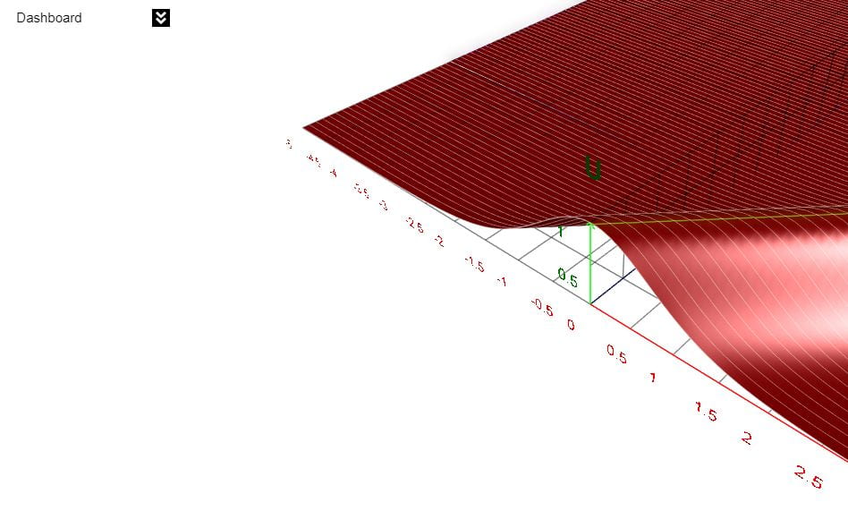
Here’s the colab worksheet. First, notice the magnitude for each complex number. Second, although not shown here, apply modulus 6 to all the real part of “z”. Third, also not show here, plot the real and imaginary numbers of z.

There’s something really beautiful hidden in the Riemann zeta.

EDIT Star Date: 1461.3 – Tu mir leid leute. Normally, I’d keep mistakes but the edit made on star date 1461.1 was just too embarrassing. Since autumn semester starts tomorrow, there may be a pause between posts. Here’s something interesting I have found in this rabbit hole.

Let
$$a,b,c \in \mathbb{N},\ p\ a\ prime,\ and\ Q\ be\ the\ quaternion\ multiplication\ operator.$$
Then for all
$$a,\ there\ exists\ some\ b\ and\ c\ $$
such that
$$[K]\ \ Re[(a +bi)(a\pm ci)]\ =\ p$$
and
$$[M]\ \ Re[Q[(a +bi)(a\pm ci)]]\ =\ p $$

Here’s the link to the colab sheet. As you can see from the first image, the quaternion multiplication in equation M is pretty interesting. Out puts are at bottom of sheet.

I’ve been on a few unreachable math journeys but this is the most interesting. Probably won’t do much during semester but if I have update, I’ll post it here.

EDIT Star Date: 1450.8 – If “a” is a prime, then for all “b” ( <=a )there exist a "c" such that "K" is true. Also, for all "a" there exist a "c" when "b"="a"-1 to make "K" true. Which mean "c" is the key. Finding "c" will unlock many doors. (a, b, and c are still positive integers)

EDIT 08/08/2021 – Star Date: 1450.3: For convenience, the function below will be referred as “K”. For every “a”, there exists a combination of “b” and “c” such that “K” is true. For the time being, to keep things interesting we’ll keep “b” and “c” less than “a”. If “a” is a multiple of a prime “p”, then “b” or “c” cannot be a multiple of “p”. The latter is a generalization of the comment made on 8/5.

EDIT 08/05/2021 – THE FOLLOWING CASES ARE NOT TRUE. Although, majority of the outputs are primes, there are some instances where it isn’t. However, not all is lost. Upon deeper investigation, it appears when “a” is even, “b” and “c” has to be odd. When “a” is odd, “b” and “c” could be either odd or even. Furthermore, the combinations of “a”,”b”, and “c” in the below format can produce all the primes. Just need to find the right combinations.

Case #1:
Suppose $$a, b, c \in \mathbb{Z}^+, \, let\, b = a – 1\, and\, c + b = a.$$
$$Then\, Re[(a +bi)(a\pm ci)] = prime. $$

Case #2:
Suppose $$a, b, c \in \mathbb{Z}^+,\, and\, a\, is \,odd, let\, c = b – 1\, and\,c + b = a.$$
$$Then\, Re[(a +bi)(a\pm ci)] = prime. $$

Here’s the link to the Colab notebook

EDIT 08/05/2021: Made the code in the Colab notebook a bit more efficient and readable. It is still inefficient in terms of algorithm because of redundant outputs, particularly a few in the beginning, but I left it that way to showcase both cases and its pattern. Also, there’s when a=b=c= 1, the output is not a prime.

TODO:
[] See if there is a general case.
[] Verify output; check against known prime lists, check if this abide the prime number theorem.
[] Find proof.
[] See if there is correlation between signals, Reimann Zeta and prime factorization.

Disclaimer: As stated above, this is not a serious post about a VERY SERIOUS subject. It’s just something I noticed while working on something else. However, I do plan to revisit this once my other projects is done or has wind down.

Was able to port the dynamic grid I made in babylon into google colab with a simple python wrapper over javascript. No need to write whole new python module. It’ll be easy to update when babylon upgrade. This will be helpful when WebGPU get released. For now, this method would be relatively easy to visualize “simple” ODE and PDEs. Hopefully, I could get a demo done before spring semester starts.

There are a few visualizers out there that utilizes threejs but it’s not too configurable or extensible. This route utilizes the full capability of the babylon library.

The colab isn’t fully ready but anyone can play with whatever is there now.

Colab: https://colab.research.google.com/drive/1cEvQXJ0O3hjOpP3gkiRfkOfu0OClkjJs?usp=sharing
Github: https://github.com/brot-senpai/pde