excel

If you have never used Excel’s “Insert a Table” function, you may not realize how much easier it can make your life. Here are some tips and tricks tables allow you to do.

How to Insert a Table

Select the data you want to turn into a table (remember the CTRL-SHIFT-END trick from my previous blog on Excel tricks and tips). Under the Insert menu tab, click on the Table icon and then click OK on the Create Table box that pops up.

Naming the Table and Quick Formatting Styles

Now you will see a new menu tab: Table Tools > Design. On this tab, rename the table something more meaningful than Table1. A meaningful name will be very helpful if you use the table as a basis for a chart or pivot table later on.

You can also select another design for your table. I recommend the simpler designs to make reading your data easier on your users, but there is certainly a wide selection available. If you want a specific look, you can create your own style from scratch or from a duplicate of one that is there.

Calculating Sums

One of the nicest features of the newly created table is the ability to calculate sums for filtered data. In a regular data range, the grand total is always the total of all the rows, filtered or not. But an Excel table will recalculate to show the total of visible rows only.

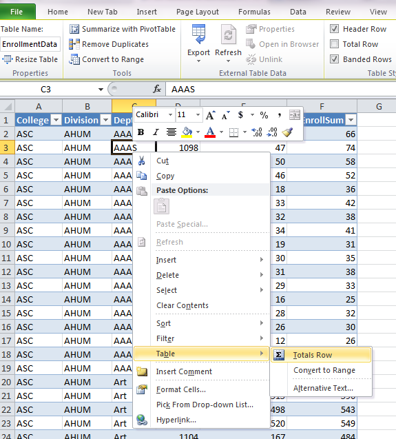
First create a totals row by right-clicking anywhere within your table. Select Table > Totals Row from the menu that appears.

A total row will be created at the bottom of the table. You can add calculations at the bottom of each column selecting from a variety of options.

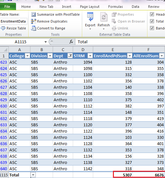
Once you create the total row, it will update every time you choose to filter your table. The table below is filtered for a single department and the totals have updated to only include the data that is show for that department.

Sorting and Filtering the Data

When you convert the data to a table in Excel, it automatically adds the sort-and-filter arrows. This makes filtering or sorting by one or more columns a breeze. Click the down arrow and select the sort or filter you desire. Any column with a filter will show a filter icon instead of the down arrow. This makes it easier to remove the filter when you are ready to look at the whole table again.

If you decide you don’t want any filters, they are easy to turn off. Click anywhere in the table, then on the Data tab click Filter. The down arrows disappear and none of the data is filtered anymore. Click Filter again to get the sort-and-filter arrows back.

Formulas in a Table

Adding a column of formulas to a table is a breeze with Excel tables. As with rows, adding a new column is as simple as adding any text or formula to a cell adjacent to the table. If you type in a formula at the top of your table, Excel will not only format the new column, but also copy the formula down the entire table.

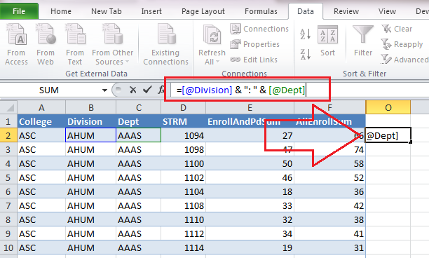
Here I have typed in the formula, but I haven’t clicked enter yet. Notice that Excel uses the column names instead of the usual cell reference number. You create the formula the same way as you would in a normal range by clicking on the cells you want to include. Excel is smart enough to substitute the[@ColumnName] format for the cell reference.

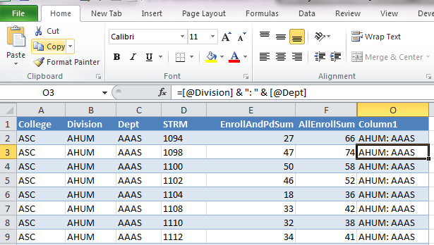
Here is the view after I hit the Enter key.

Now I can rename the column something more meaningful than Column 1.

The copy down functionality is terrific, but even better is what happens if you need to delete all the rows and paste or type new data into the table. Excel remembers the formula and recalculates the column automatically. You never need to retype the formula as long as you have the table.

Creating a Chart

Creating a chart from the new table makes the chart much more dynamic than if it were based on a range. The chart will automatically include new rows of data. It will also update based on the filter you apply which makes it great for investigating trends. When you select the data range for your inserted chart, use the table name instead of highlighting the rows. Since you gave your table a meaningful name, this should be much easier than choosing the range.

Reverting Back to Normal Range

If at some point you want the extra table features to go away, it is easy to revert back to a normal range. Click anywhere inside the table, then select Convert to Range from the Table Tools > Design menu tab and the nifty functionality of tables goes away.

The following tips are fairly simple things you can do to make Excel less time consuming. They are so simple you might wonder why no one has told you about them before!

Quick Sums and Averages

Suppose you are working on a spreadsheet in Excel, and you want to quickly check that the column of numbers you just entered matches the total you are expecting. No need to click the Quick Sum button, just highlight the cells you want to total and look at the bottom of your screen. Excel automatically creates an Average, Count and Sum calculation every time your highlight cells.

Shortcut Keys for Selecting

Excel has a lot of short cut keys that can really make your life easier if you have to do repetitive actions. You can find a partial list at here. For this post, I wanted to spotlight two ways of selecting large portions of a spreadsheet quickly. When I’m working in Excel, I often want to select all or most of the spreadsheet. A quick way to make this selection is to click on the top left cell in the block you want to select then use CTRL SHIFT → ↓.

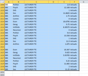
However, using the CTRL SHIFT → ↓ is great only if you have a complete block with no missing rows or columns. To make sure you get everything, use CTRL SHIFT END and the highlighting will extend all the way to the last used cell in the worksheet.

Transpose a Table

Suppose you have a table in Excel and you want the columns to be rows and the rows to be columns. There is a “quick and dirty” way to do it quickly.

1) Select the data you want to transpose. Copy.

2) Select a blank cell in your worksheet where you want the transposed table to appear; select the arrow for Paste from the Home tab. The Transpose symbol is in the second row, third column of the Paste options.

Voila! Your data has been transposed. The downside of the quick and dirty version is that the newly created table is not linked to the original table. If you change something in the original table, it will not be updated in your transposed version. There is a way to transpose while keeping that connection, but that will have to wait for a later post since it is a lot more complicated.

Display Formulas Instead of Values

Sometimes when you create a complex spreadsheet with a lot of calculations, it can be helpful to view all the calculations in the spreadsheet instead of the results of the calculations. This is particularly helpful when you are trying to track down an error.

Excel provides a shortcut to quickly do this: CTRL `.

The ` grave accent key is located at the top left of your keyboard with the tilde.

Press once and the spreadsheet displays the formulas; press again and you get the results to appear again.

Getting the Most from the Quick Access Toolbar

If you use Excel a lot, you may find yourself using a specific command over and over again. Paste Values is one I use a lot and I’ve frequently wished for a shortcut key to make my life easier. An underused trick in Excel will allow you to create such a shortcut quickly and easily.

1) Click the down arrow at the right of the Quick Access Toolbar.

2) Click More Commands…

You can limit the number of commands you see by selecting “Commands Not in the Ribbon” from the “Choose commands from:” drop down box.

3) Select Paste Values (or your preferred command) and Click Add.

Quick Access -Add Paste Values

By default, Excel will add this to all your documents. If you only want this shortcut to show up in the current document you can make that selection using the “Customize Quick Access Toolbar” drop down box (see the blue highlighted box above).

4) Click OK

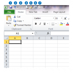
Now the fun begins. Not only can you see this one click item all the time, but if you prefer to use keystrokes, you can access by holding down the Alt key and pressing the number corresponding to the position of the icon in the Quick Access Tool Bar. In my case, I added Paste Value into the 7th position on the Toolbar so I can use Alt 7 to call on it at any time.

Quick Access - Hot Keys

Coming soon…

There are numerous tips and trick to Excel that can make your life easier. I have only presented a few here, but there will be plenty more coming soon. In the near future, we’ll take a look at the “Insert a Table” function and how this simple tool can be a truly powerful friend. Later on, we’ll be looking at creating our own simple macros for personalized short cuts. It’s easier than you think!

Ohio State nav bar

Insert a Table in Excel